Category Archives: GIS

swat 2005 源代码的编译

swat 2005源代码是可以从官方网站上下载到的。尝试了gfortran 编译,首先删除了*.mod,使用 gfortran –c modparm.f 重新生成 parm.mod。在main.f里注释了第一行,即include ‘modparm.f’。否则会出现重复定义的问题。最后编译,可以成功,但在运行时出现 Fortran runtime error,大致是从文件里读取end of file之类的错误。

安装了intel fortran 编译器,用的是官方的30天试用版。在visual studio 2010里建立了fortran console application项目,将swat 2005里的全部*.f 加到里面。同样重新生成 parm.mod,并修改了main.f (同上),编译,试运行,可以用。

ArcGIS 10 license

Arcgis Desktop 10安装后,D版盘里还有个Crack_LM_ArcGIS10目录,里面有Crack_LM程序,运行后生成c:Cracked License Manager 10目录,以及将一个afcore库copy进arcgis相应的位置。不必安装arcgis10自带的License Manager。

注意,除了lmgrd.exe要解除firewall,arcgis.exe也要解除,否则不能使用。

破解License的目录(c:Cracked License Manager 10),不能改名。如果不中意此名,一定要修改的话(以修改成ArcGIS License Manager 10为例),可以用以下方法:

1. 任务管理器里找到lmgrd.exe, 结束之。arcgis.exe因为是lmgrd.exe调用,会自动结束。

2. 在资源管理器里,将Cracked License Manager 10 修改为ArcGIS License Manager 10。

3. 用记事本打开此目录下的start_lic_mgr_invisible.vbs,将其中的Cracked License Manager 10 改为ArcGIS License Manager 10。保存关闭。

4. 用记事本打开start_server_license.bat,将Cracked License Manager 10 改为ArcGIS License Manager 10。保存关闭。

5. 点击,开始 > ArcGIS License Manager 10 CRACKED > ArcGIS License Manager 10 CRACKED 会提示 lmgrd.exe 和 arcgis.exe 的security alert,全部 allow access。

6. 打开 arcmap 10 测试 是否正常运行。

7. 到防火墙设置里,允许通过列表,去掉 原先在 cracked … 目录下的arcgis.exe 和 lmgrd.exe(列表名叫Acresso Software Inc.)。

Done!

Windows 7 多用户模式下安装AVSWAT 2005

1. 安装 arcview 3.2,安装完后,不要重启,打开arcview 3.2,键入注册码
2. 安装spatial analyst 2.0,安装完后,不要重启
3. 打开控制面板,将区域与语言里的格式,从中国改成 英语(美国),位置处的中国
可以不改。
4. 安装arcview, SA 都请安装在默认目录下,即不包括空格
5. 将avswatx的安装包解压缩到 c:esri 目录下的avswatx里。
6. 用管理员权限(重要!)打开arcview 3.2,打开 c:esriavswatx下的
setup.apr,将开始avswatx的安装。
7. 选择 for all users,在我安装时,选 only for me ,安装可以,但在装载swat的
时候提示注册表的 avswatx/swatdatabase等找不到。
7.1 重启,否则在使用arcview时可能提示 ntfont.c 错误等。
8. 以当前用户权限打开 arcview 3.2,在extensions里选择 avswatx extendable 和 spatial analyst 扩展。
9. 可以正常运行了。

天地图初印象

10月21日国家测绘局宣布中国区域内数据资源最全的地理信息服务网站“天地图”(www.tianditu.cn)正式开通,提供地图模式、影像和三维模式。

敲入网址,所谓正式开通,也只是测试版。

接着出来的友情提示,建议大家使用微软的IE浏览器,并更新到IE7,8。让人奇怪是不是测绘局跟微软是不是有什么协议。现在IE市场份额节节下跌,Firefox, Chrome, Safari 都做的这么出色,占有越来越多的市场的时候,这个东东还推荐使用IE,而且三维模式是必须在IE内核下才能用。

第2个友情提示,就更是让人哭笑不得。

image

用户账户控制是Windows Vista以上版本的一个重要安全机制,它居然要让大家关闭掉。幸运的是,没有要求大家将杀毒软件也关掉。反正中毒了,是不需要天地图负责任的。其实我看到这个提示,已经失去继续使用的兴致了。

勉强再试一下放大缩小。载入的速度明显没有google map快,漫游也不是很顺畅;切换到影像,只看了一下兰州地区的,灰蒙蒙的,而且只有很粗分辨率的;三维在chrome之下则无法使用。

全部的功能貌似没有超出google map;换句话说,天地图相比 google map甚至 baidu map,优势体现在哪里?

Using ArcGIS to prepare Sub catchment file for TopMODEL

Zhuotong Nan ([email protected]), CAREERI/CAS

TopMODEL is a conceptual hydrological model which was initially released in 1979 but is still widely used today especially in a watershed simulation with sparse observations.  TopMODEL uses topographic index (TI) to calculate water flow. There are already some tools developed for TI computation. Here I want to present a method using ArcGIS.

There is a similar work at http://soilandwater.bee.cornell.edu/Courses/GIS/TI.ppt. What I will present will be more than it.

1. We have  a DEM which is large enough to cover our study area. The DEM “Heihe_SRTM.img” is subset from the SRTM 90m data which is in lat/lon coordinates (WGS84).

image

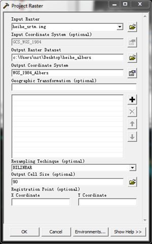
2. Open ArcToolbox, go to Data Management Tools > Projections and Transformations > Raster > Project Raster.

image

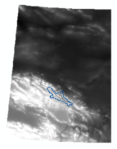
Here use bilinear to interpolate the input raster to a 90m resolution grid in the Albers equal area projection.  The resulted raster is “heihe_albers”.

image 

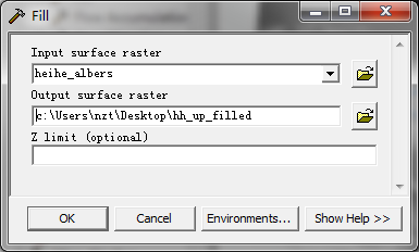
3. In ArcToolbox, Spatial Analyst Tools > Hydrology > Fill, to fill up the possible sinks, resulting “hh_up_filled”.

image

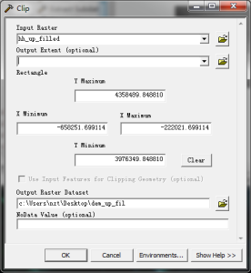
4. In ArcToolbox, go to Data Management Tools >Raster > Raster Processing > Clip, to make the filled DEM smaller, because the next steps are very computation intensive. “dem_up_fil” is created.

image image

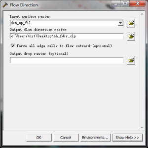
5. Hydrology > Flow direction. Note, use the filled DEM. flow direction file is “hh_fdir_clp”.

image

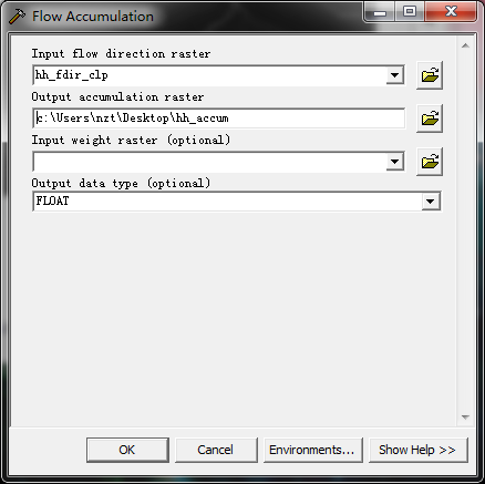
6. Hydrology > Flow Accumulation to compute “hh_accum”

image

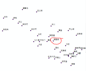
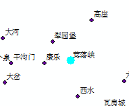
7. open hydrosta.shp. this is a hydrological station location shapefile. We use the red line surrounded site as the watershed outlet.

image

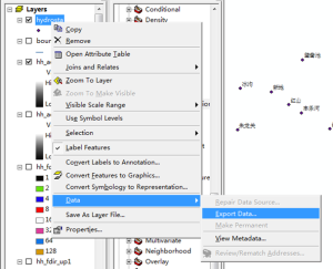
8. use the “select feature” to select the desired site

image image

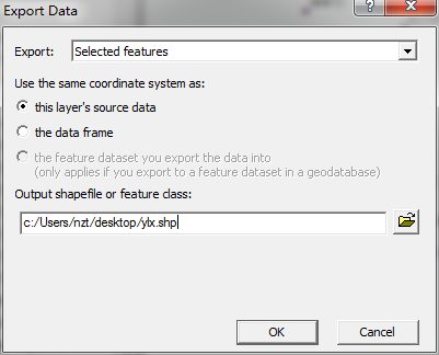
9. export to a separate file. the exported ylx.shp now is in same projection as hydrosta.shp which is lat/lon.

image image

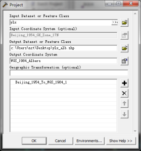
10. Data Management Tools > Projections and Transformations > Feature > Project. save as “ylx_alb.shp”.

image

the output coordinates can be imported from the heihe_albers raster.

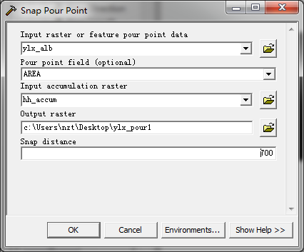
11. Hydrology > Snap Pour point. Carefully select the snap distance which is in map units. The result is “ylx_pour1” grid.

image

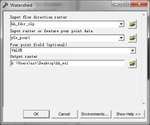
12. Hydrology > Watershed to delineate the watershed. Now we have “hh_ws1”.

image

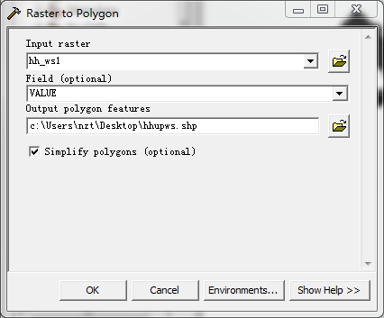
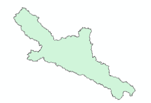
13. ArcToolbox > Conversion Tools > Raster to Polygon to create “hhupws.shp”

image image

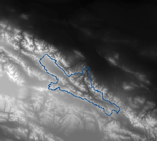
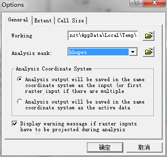
14. Open Spatial analyst toolbar (right click on the blank space of menu bar, select Spatial Analyst), set Spatial Analyst > Options > Analysis mask to hhupws (the watershed boundary polygon)

image

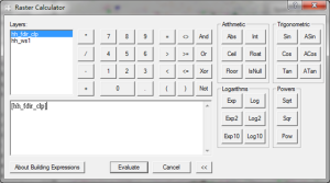
15. Spatial Analyst > Raster Calculator, double click hh_fdir_clp, and then click Evaluate. This will make the hh_fdir_clp masked by the watershed boundary.

image

Make the generated Calculation layer permanent (right click the item in the TOC, Data > Make Permanent…). Save as “hh_fdir_up1”.

Do same to dem_up_fil; dem is clipped to “dem_upstr1”.

Do same to hh_accum to generate “hh_accum_clp”

image image image
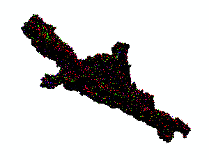
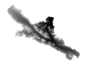
hh_fdir_up1 (left), dem_upstr1 (middle) and hh_accum_clp (right)

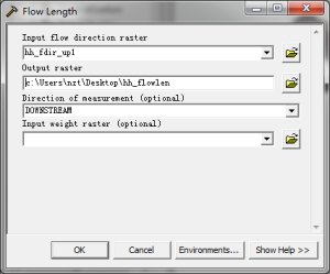
16. Hydrology > Flow Length

image

the flow length raster “hh_flowlen” is used to calculate channel levels in the SUBCAT file.

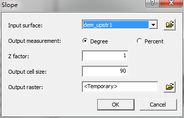
17. Spatial Analyst > surface analysis > Slope

image

save the slope file as “Slope_filldem”

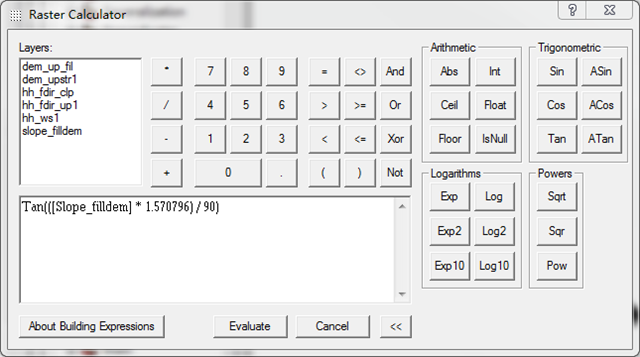
18. Spatial Analyst > Raster Calculator

image

use “Tan(([Slope_filldem] * 1.570796) / 90) ” to calculate tangent of slope radians

save to “tan_slope1”

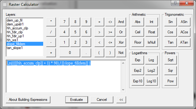
19. Same in Raster Calculator

Calculate TI by typing “Ln((([[hh_accum_clp]] + 1) * 90) / [[slope_filldem]] )”

image

save to “ti1”

Now we have data ready. What we do next is to classify data and make data formatted to fit what Topmodel requires.

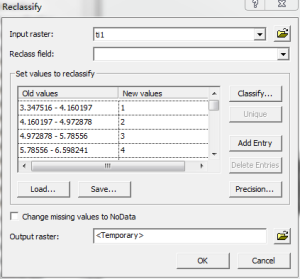
20. Select ti1, then click Spatial Analyst > Reclassify … In the window, click Classify, select Equal Interval as the method, set 29 as the classes, click Ok to accept it. Other classification methods also can be used for your cases. You also can set more classes. but keep in mind that the TopModel version might be have limitation on classes.

image

click “Save…” , save the classification schema to “ti_table” as info table

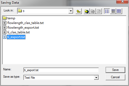
Click ok to classify the continuous TI grid. a new layer “Reclass of ti1” is added to TOC. select it and right click to bring up the context menu. Open Attribute Table, and then Options > Export all records to “ti_export.txt”.

image

Note, the Save as type should be selected as “Text File”. It might not work if you only specify an “.txt” extension.

Do same to the hh_flowlen. classify it to 9 classes. and export the data to “flowlen_export.txt” in a text format. The classification schema is saved to “flowlen_table”.

21. In ArcGIS, click Add data to adding flowlen_table and ti_table to the ArcGIS session.  Right click on each item, open the table, and export all data to text files, here, “flowlength_clas_table.txt” and “ti_clas_table.txt”, respectively.

image

22. Open Excel. drag “flowlength_clas_table.txt”, "ti_clas_table.txt”, "ti_export.txt”, and “flowlen_export.txt” to Excel.

In each Excel workbook, select the first column, click “Text to Columns” in the data tab of Excel 2007. in the earlier version, there is also similar commands.

select comma as the delimiter, click finish.

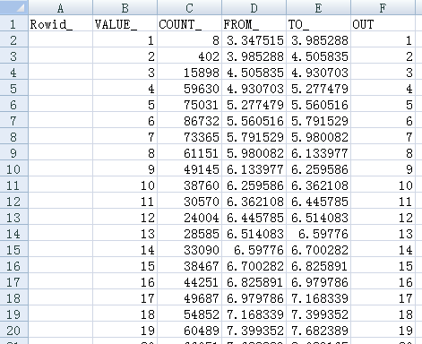
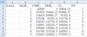
Copy “From_”, “To_”, “Out” columns in class schema files, append to ti and flowlen export data workbooks respectively. This step is to combine the schema to actual data. after appending, close the two class table files (“flowlength_clas_table.txt”, "ti_clas_table.txt”) without saving changes. Now we have something like that,

image image
The combined ti_export.txt workbook(left) and the combined flowlen_export.txt workbook (right)

23. In the ti_export.txt workbook, select the “OUT” cell, click reverse order command image .

Right to the “OUT” column, add “Area”, and then “TI”. 

In the cell below the title “Area”, type: =c2/sum($c$2:$c$30).  this will calculate the fractional area. Note, $c$30 indicates the last low of the data. You might change it accordingly when you have different classes. Copy this cell to propagate through the Area column.

In the cell below the title “TI”, type: =D2. Copy this cell to propagate through the Area column.

Insert a new row right below the header row where we set area to 0, and ti to “=E3” (the largest TI). like below in this time,

image

Save the result to a new Excel file, say, “ti_ready.xlsx”.

24. In the flowlen_export.txt workbook, right to the “OUT” col, add “area”, “accum_area”, and “dis” in the next two cells.

use “=C2/SUM($C$2:$C$10)” to calculate the area column; note, $c$10 is the last data line. change it accordingly.

use “=SUM($G$2:G2)” to calculate accumulative area for the accum_area column;

use “=e2” to calculate the dis column.

copy those formula to other rows.

insert a new line immediately below the header line. type 0 and 0 for accu_area and dis.  if this is a subcatchment, set the distance from the outlet of the entire catchment to dis here.

looks like as below,

image

save the excel to “flowlen_ready.xlsx”

close ti_export.txt and flowlen_export.txt, no need to save changes.

Note, we do not need to reversely sorting data which is different from the ti case described above.

25. copy “area” and “ti” in the ti_ready.xlsx (without header) to the proper section of the SUBCAT file.

copy “accum_area” and “dis” in the flowlen_ready.xlsx (without header) to the proper section of the SUBCAT file.

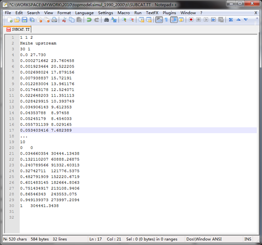
in this case, the total ti increments are 30; the total channel levels are 10. looks as below,

image

For the demonstration purpose, we abbreviate 30 ti increments.

A Lab for using the PIHMgis and PIHM model (II)

Zhuotong Nan (南卓铜, [email protected])

DEM processing

In this part, we will show you how to delineate a watershed with inputs of DEM(Digital elevation model) and outlet location. Watershed delineation is necessary for any distributed hydrologic model. Although hydrologic models use different software to implement the delineation, the underlying idea and steps are generally common.

1. Open PIHMgis by double clicking the PIHMgis_v2.0.0 shortcut created in the previous section.

2. Enable PIHMgis.

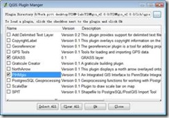
Open Plugin Manager… in the QGIS Plugins menu, tick the PIHMgis item (Figure 3), and press Ok.
clip_image002

Figure 3 QGIS Plugin Manager

Now the PIHMgis toolbar appears as shown in Figure 4.

clip_image004

Figure 4 the PIHMgis v2.0.0 toolbar

3. Load DEM to PIHMgis for displaying.

Layer > Add a Raster Layer…, select lab3.shale.hillsDEMsh_elev.asc.

This DEM file is in ESRI ASCII grid file format. If you have files in ESRI binary grid format which is a proprietary format, you need to convert them to ASCII format by using some ArcInfo command or by some third party tool, such as gdal_translate available from the GDAL website at http://www.gdal.org/.

The map view of the DEM file looks like as following (Figure 5),
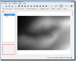
clip_image006

Figure 5 DEM map view in QGIS

4. Save as a QGIS project. File > Save Project As…, in the Save As dialog, navigate to the directory of lab3.shale.hills, type “sh” for the file name, and then click Save.

Note: During following steps, please save the project frequently. If the project is crashed, you can restore to the previous session by open the project you saved.

5. Fill pits.

Question: Why do we need to fill pits for a DEM file prior to further watershed delineation?

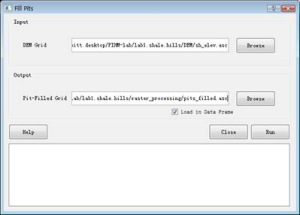
Click the small arrow next to the Raster Processing on the PIHMgis toolbar and then select Fill Pits. This will bring up the Fill Pits dialog (Figure 6).
clip_image008

Figure 6 The Fill Pits interface

Select sh_elev.asc as the input DEM grid and name the output pit-filled grid as “pits_filled.asc” under the “raster_processing” directory as shown in Figure 6. Press Run to start the pit filling process. Click “Close” to dismiss the dialog after the process is done. The pit-filled DEM will automatically be loaded into the QGIS data frame.

6. Calculate flow direction and flow accumulation.

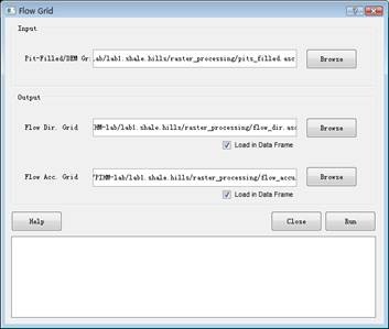
Use the command Raster_Processing > Flow Grid to open the Flow Grid window (Figure 7).

Set pits_filled.asc as the input; flow_dir.asc and flow_accu as the output flow direction grid and flow accumulation grid respectively, also under the raster_processing folder.

Click Run to start the processing. After done, click Close.
clip_image010

Figure 7 Flow Grid

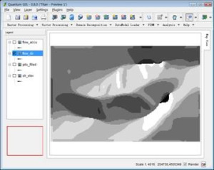
Both flow_accu and flow_dir are shown in the QGIS map view (Figure 8).

Note: the direction codes are following: 1 – east, 2 – North east, 3 – North, 4 – North west, 5 -West, 6 – South west, 7 – South, 8 – South east.
clip_image012

Figure 8 Flow direction generated by PIHMgis

Tip: Within the QGIS framework, visibility of a GIS layer can be switched using the table of contents on left.

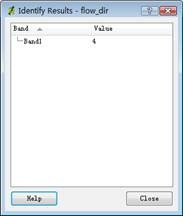
Tip: The identify tool clip_image013 can be used to identify features by clicking on them in the right map view panel. For example, click on the flow_dir item in the table of contents to make it selected, and then use the identify tool to click over the map view, the Identify Results dialog will pop up and show the value of the clicked feature (Figure 9), here, value of 4 means the point of interest has a flow direction towards north west.
clip_image015

Figure 9 Identify results

7. Generate stream grid

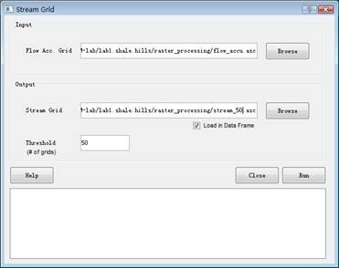
Select Raster Processing > Stream Grid to make the Stream Grid dialog visible, set the flow accumulation grid generated in previous step, i.e., flow_accu.asc, as the input grid, and then set output stream grid to stream_800.asc with a threshold value of 800 (number of grids). Press Run to generate stream grid (Figure 10).
clip_image017

Figure 10 Generate stream grid with a threshold value of 50.

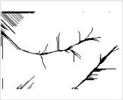
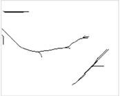
Don’t close the Stream Grid window. Set thresholds to 300 and 800 respectively to compare the resulting stream grids (stream_300 and stream_800 accordingly, Figure 11) and run again.
clip_image019clip_image021clip_image023

Figure 11 The generated stream grids with thresholds set to 50, 300 and 800. (left: 50, middle: 300, right: 800)

Close the Stream Grid dialogue by clicking on the Close button.

Question: How to determine an appropriate threshold for a watershed of interest?

8. Generate the stream order grid (known as Link Grid in PIHMgis)

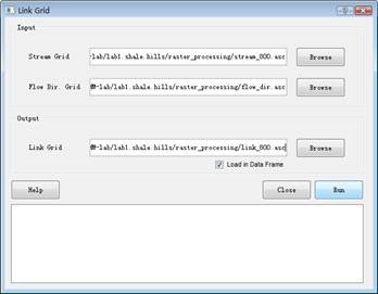
Select Raster Processing > Link Grid to pop up the configure interface (Figure 12). Select stream_800.asc as the input stream grid and flow_dir.asc as the input flow direction grid, and set the output link grid name to link_800.asc (saving to the same raster_processing folder). Click Run to begin processing. After done, the link grid will be shown on the map view panel if the Load in Data Frame option is checked.
clip_image025

Figure 12 Generate a stream order grid

9. Create a vector file of stream network

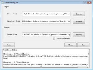
Select Raster Processing > Stream PolyLine to make the interface appear (Figure 13). Set inputs with stream_800.asc and flow_dir.asc generated by previous steps and set the name of the output stream polyline file to str800.shp. Click Run to process it after parameters are specified.
clip_image027

Figure 13 Create a vectorized stream network

10. Generate catchment grid and its corresponding vector file

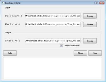
Select Raster Processing > Catchment Grid to bring up the catchment grid generation interface (Figure 14). Set Stream Link Grid to link_800.asc, Flow Dir. Grid to flow_dir.asc, and output Catchment Grid to “cat_800.asc”. Both input and output files are located in the raster_processing directory.

Click Run to start calculating the catchment grid. Click Close to dismiss the dialog.

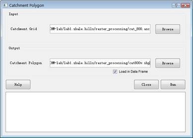
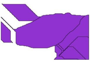
Select Raster Processing > Catchment Polygon to display the interface for converting grid catchment file to vector (Figure 15). Set input to cat_800.asc and output to cat800v.shp. Run to start the processing and Close to dismiss the window. The resulting catchment polygons are shown on Figure 16. Note: the color to render the polygons might not be same as that on the Figure 16, as it is determined by QGIS automatically.
clip_image029

Figure 14 Catchment grid generation interface
clip_image031

Figure 15 Convert catchment grid to vector
clip_image033

Figure 16 Resulting catchment polygons

11. Extract the watershed boundary of interest

The current PIHMgis version 2.0 does not provide such a function to clip the watershed boundary under study and stream network within it. We need to do this by help of other GIS software such as ESRI ArcInfo, or by using QGIS editing capability demonstrated below. In the future version of PIHMgis, this functionality will be implemented. To determine the boundary of a watershed, the outlet location should also be specified.

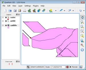
Open QGIS 1.0, load cat800v.shp and str800.shp generated in previous steps to the data frame using Layer > Add Vector Layer…, and then load outlet.shp, which contains outlet location. The view now looks like Figure 17.
clip_image035

Figure 17 QGIS 1.0 with stream network, catchment polygons and outlet layers loaded

Click on cat800v within the table of contents to make it the current layer. Use “Select Features” tool (Figure 18) to select the watershed polygon of interest (Figure 19). The selected polygon is now in yellow. If the tool is invisible, just drag the toolbar to a new place to make fully appeared.

Students are advised to have a look at all built-in toolbars, making them familiar with all those often-use tools.

clip_image037

Figure 18 The Attributes toolbar

clip_image038

Figure 19 Select the watershed of interest

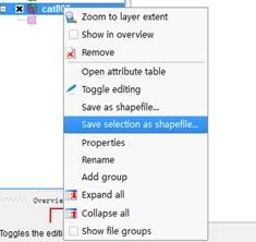
Right click the cat800v item and select “Save selection as shapefile…” to save the selected polygon (Figure 20) to a new shapefile, here, “cat800v_sel.shp”, under the “raster_processing” folder. If you are required to select a project, click OK to use the default one.

Note: The default project probably is not correct, but does not matter with following operations. You can change the project in a layer’s property window later.
clip_image040

Figure 20 Save selection as a new shapefile

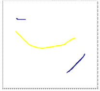
Similarly, select the corresponding stream from str800 and save as a new shapefile “str800_sel.shp” (Figure 21), also into the “raster_processing” folder. If you are required to select a project, click OK to use the default one.
clip_image042

Figure 21 Select the corresponding stream, shown in yellow.

Load str800_sel and cat800v_sel into the QGIS map view. Drag layers up or down to rearrange layers’ visibility. Uncheck str800 and cat800v to hide them. Now the map view looks like Figure 22.
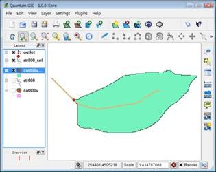
clip_image044

Figure 22 Load str800_sel and cat800v_sel and hide str800 and cat800v

Make str800_sel disappear. Select “cat800v_sel” layer, and use “zoom in” tool (the one w/ magnifier icon and a plus symbol shown in Figure 23) to enlarge the area near the outlet. Click “Toggle editing” tool (the one w/ pen icon shown in Figure 23) to make the current layer editable (Figure 23). Now the other tools on the Digitizing toolbar are also available when the layer enters into edit mode. The tools may be hidden, in this case drag toolbars to a blank place to make all tools shown.
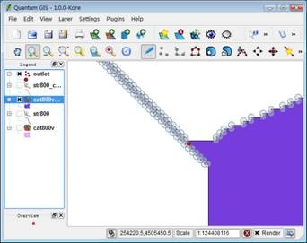
clip_image046

Figure 23 cat800v_sel in edit mode

Click the Split Features tool. Draw a curve to cross the outlet so as to split the whole polygon. Right click to finalize the curve; the Split Features will then split the polygon. Click the “Toggle editing” again to make the layer back in the normal view mode. Make sure saving it if you are asked to save the features.

Use “Select Features” tool to select the large polygon right to the outlet. If the previous operation has been done successfully, only the large part will be selected and the upper left part remains unselected. Save the selected polygon to a new shapefile named “cat800v_clip.shp”. Load cat800v_clip to the map view. It now looks like as shown on Figure 24.
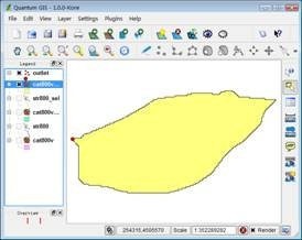
clip_image048

Figure 24 Clipped watershed boundary

Similarly, we also split the str800_sel.shp. Make it visible and editable, draw a curve to split it across the outlet, save the operation, and then export the desirable line (on the right) to a new shapefile, “str800_clip.shp”. (Figure 25)
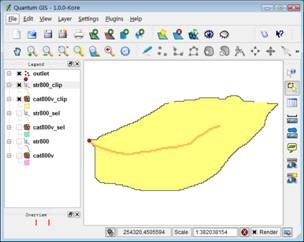
clip_image050

Figure 25 Clipped stream network

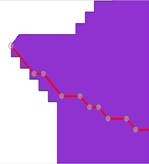
Zoom in the outlet area, and carefully edit the stream polyline making its end node locate on the watershed edge. However no necessary exact alignment is needed. Tools for vertex editing are shown in Figure 26. The final stream line looks like as in the Figure 27. Save the stream file after done.

clip_image052

Figure 26 vertex editing tools. Left: move vertex; middle: add vertex; right: remove vertex
clip_image054 clip_image056

Figure 27 Align the end node of stream line to the boundary. Left: original; right: edited

Close QGIS 1.0.

A Lab for using the PIHMgis and PIHM model (I)

Zhuotong Nan (南卓铜, [email protected])

Set up work place

1. Download PIHMgis version 2.0 from the URL:

http://www.pihm.psu.edu/PIHMgis_v2.0.0/PIHMgis_v2.0.0.zip

Download Shale Hills PIHMgis data files from the URL:

http://cid-0ea641a5a7f665a1.skydrive.live.com/self.aspx/Public/shale.hills.pihmgis.data.zip

Download qgis.1.0 from the URL:

http://cid-0ea641a5a7f665a1.skydrive.live.com/self.aspx/Public/qgis.1.0.zip

Note: The current PIHMgis v2.0 is built with QGIS 0.8 preview version and cannot run with QGIS 1.0 because APIs of those two version are inconsistent. The stable QGIS 1.0 version provides us a much better user interface and richer functionality than version 0.8. We will use QGIS 1.0 editing functions to manipulate vector data. The development team of PIHMgis is working on the migration to QGIS 1.0, which might be available in near future.

2. Make a directory “PIHM-lab”, and then extract “PIHMgis_v2.0.0.zip” to this directory. Go to this PIHMgis_v2.0.0 folder, locate “PIHMgis_v2.0.0.exe”, make a shortcut and rename the shortcut to “PIHMgis_v2.0.0”, and then copy this shortcut file to the directory “PIHM-lab” (our lab root directory).

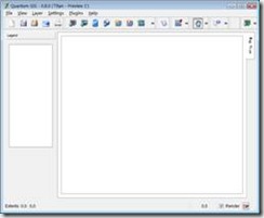
Clicking the shortcut will bring up the Quantum GIS (QGIS) window, as shown Figure 1. Click “X” to close QGIS.

clip_image002

Figure 1 the QGIS 0.8 preview version interface coming with the PIHMgis. Note, the interface might be shown in different language if your computer locale is not set to English.

3. Create a directory “lab3.shale.hills” under “PIHM-lab”. Extract “shale.hills.pihmgis.data.zip” to the “lab3.shale.hills” directory.

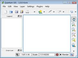
4. Extract qgis.1.0.zip to the directory “PIHM-lab”, go to “qgis.1.0bin”, make a shortcut “qgis” for qgis.exe under this folder, and then copy this shortcut to the directory “PIHM-lab”. Click the qgis shortcut to open it, making sure it can work. It looks like Figure 2.

clip_image004

Figure 2 the QGIS 1.0 interface

Land cover数据Goode格式在ArcGIS中的访问

南卓铜 ([email protected])

一些有名的Land cover数据集并没有使用通用的GIS格式,比如在以下链接,

http://www.geog.umd.edu/landcover/tree-cover-poster/download.html

下载broadleaf Layer,gzip解压缩后为 694,417,920 bytes,扩展名为.img,但不同于Erdas Imagine .img格式。

据介绍Goode binary file是plain binary,即相当于BSQ (Band sequential),其metadata有以下信息:

40031 pixels by 17347 lines,且是8bit unsigned integer,应当总大小为 694,417,757bytes,而解压缩后的大小大了163bytes,目前我还不知道原因。

根据metadata信息,可以添加头文件,broadleaf.hdr,内容如下,

nrows      17347
ncols     40031
nbands     1
nbits     8
layout     bsq
skipbytes     0
ulxmap     -20015500.000
ulymap     8673500.000
xdim     1000
ydim     1000

将broadleaf.img改名为 broadleaf.bsq,在ArcGIS中才可以正常访问,也可以导出为其它格式,比如Grid。不过注意其空间参考系仍为unknown。在ArcCatalog中打开其属性页,在spatial reference中选projected coordinates/World/Goode Homolosine (Land).prj。可以将bsq设置为 Goode投影。

如果希望转换成其它常用格式,

image

上图将bsq转成ESRI binary grid格式。图形化结果如下图。

image

在Workstation下好像没有找到Goode投影,但在Desktop下可以找到.prj。因为如果bsq是unknown时,导成esri grid,在ArcCatalog里对grid进行定义投影(属性->define spatial reference),没法子定义到Goode投影,很奇怪。所以这里,我是先对bsq定义投影,再转成grid。此外,通过ArcToolbox的Data Management下的projection define来做,也是可以。

ArcGIS Identity command “Number of shapes does not match the number of table records” error

When I run Identity_analysis in ArcGIS command windows against geodatabase, a message of something like "Number of shapes does not match the number of table records" popups. The error continues even if you reinstall the ArcGIS whenever using the Identify command.

Solution: go to c:documents and settingsyournamelocal settingstemp and delete all the files (some files might be denied to access, just skip them).

ArcGIS栅格向Surfer Grid的格式转化 (Convert ArcGIS raster to Surfer GIS)

Zhuotong Nan ([email protected])

以下简单的代码实现了ArcGIS支持的栅格向Golden software的Surfer ASCII grid的格式转化。需要注意的是,ArcGIS的栅格左上为坐标原点,向下向右为正。而Surfer grid是左下是坐标原点,向上向右为正。

Here I will show a class that implements the major functionality to convert any Raster file supported by ArcGIS to Surfer ASCII grid format. The resulting Surfer grid can be read by Surfer with version 6 or higher. One point we need to keep in mind, ArcGIS raster stores data in row-major order, right and downwards being positive, while Surfer grid takes lower left corner as the original, right and upwards being positive.

using System;
using System.Collections.Generic;
using System.Text;
using System.IO;
using ESRI.ArcGIS.Geodatabase;
using ESRI.ArcGIS.DataSourcesRaster;
using ESRI.ArcGIS.esriSystem;
using ESRI.ArcGIS.Geometry;

namespace RasterToSurferGrid
{
/// <summary>
/// A wrapper class for Surfer ASCII grid file
/// </summary>
class SurferGrid
{
string id = “DSAA”;
int nx;//columns
int ny; //rows
double xlo; //the minimum X value of the grid
double xhi; //xhi is the maximum X value of the grid
double ylo;
double yhi;
double zlo;
double zhi;
List<double> data; //the grid is stored in row-major order, with the lowest row (minimum Y) first

public SurferGrid(string rasterPath)
{
data = new List<double>(nx * ny);

IWorkspaceFactory wf = new RasterWorkspaceFactoryClass();
IRasterWorkspace wk=(IRasterWorkspace)wf.OpenFromFile(System.IO.Path.GetDirectoryName(rasterPath), 0);
IRasterDataset ird = wk.OpenRasterDataset(System.IO.Path.GetFileName(rasterPath));
IRaster raster=ird.CreateDefaultRaster();

IRasterProps props = (IRasterProps)raster;
nx = props.Width;
ny = props.Height;
IEnvelope env = props.Extent;
xlo = env.XMin;
xhi = env.XMax;
ylo = env.YMin;
yhi = env.YMax;
//zlo = env.ZMin;
//zhi = env.ZMax;

//populate data
PntClass extent=new PntClass();
extent.X=nx;
extent.Y=ny;
IPixelBlock datablock=raster.CreatePixelBlock(extent);
PntClass orig = new PntClass();
orig.X = 0;
orig.Y = 0;
raster.Read(orig, datablock);

for (int y = ny – 1; y >= 0; y–)
//for (int x = 0; x < nx; x++)
{
for (int x = 0; x < nx; x++)
{
data.Add((float)datablock.GetVal(0,x,y));
}
}

//get the max, and min
double max, min;
max = data[0]; min = data[0];
for (int i = 0; i < data.Count; i++)
{
max = max > data[i] ? max : data[i];
min = min < data[i] ? min : data[i];
}

zlo = min;
zhi = max;
}

public void WriteToFile(string outPath)
{
//StringWriter sw = new StringWriter();
StreamWriter sw = new StreamWriter(outPath);
sw.WriteLine(id);
sw.WriteLine(“{0} {1}”, nx, ny);
sw.WriteLine(“{0} {1}”, xlo, xhi);
sw.WriteLine(“{0} {1}”, ylo, yhi);
sw.WriteLine(“{0} {1}”, zlo, zhi);
StringBuilder sb=new StringBuilder();
for (int i = 0; i < ny; i++)
{
for (int j = 0; j < nx; j++)
{
sb.AppendFormat(“{0} “, data[i*nx+j]);
}
sb.Remove(sb.Length – 1, 1);
sb.AppendLine();

}
sw.Write(sb.ToString());
sw.Close();
}

}

}

附件是源代码。工具的运行需要dotnet framework 2.0和ArcView以上的License运行。编译后在命令行敲入RasterToSurferGrid有使用提示。

The attached please find necessary source codes which can be compiled on your own platform. Dotnet framework 2.0 and a valid ArcView license or higher are both required to run this tool. Besides, ArcGIS assemblies for dotnet framework are required. After successful compilation, typing RasterToSurferGrid following the command prompt shows you its usage information.
RasterToSurferGrid.zip