Monthly Archives: February 2009
56年的春晚
在文学城上看到一个帖子,介绍56年春晚的一些情况。很惊讶地看到有照片是郭沫若向大家介绍钱学森、华罗庚等科学家。或者本不该惊讶的,但我的确惊讶了,我是以现在的眼光看以前那个年代。
春晚是个娱乐节目,科学家不应当露面,这些年国家领导人也不再出现了,这是个进步。
只是平时主流媒体对科学成果和科学人物的宣传极其不够。联想到现在的媒体,基本上充斥了娱乐甚至低俗内容,罕见真正有价值的东西。至少科学家,见鬼去吧,科学家本应当甘于寂寞,关在实验室,跑媒体上来干什么。
科学家应当如何自律是一个方面,但媒体的宣传导向却是另一方面,给我的印象媒体已经将大家的价值观尤其是成长的一代引到一个极其危险的地步。问问现在的小孩子吧,他们的学习对象奋斗目标都是哪些人哪些对象,我怀疑还有没有小孩会说,以后长大了要当科学家吗。
娱乐之所以被叫做娱乐,就是因为那些东西永远不能代替吃饭和发展。我不是看不起全部从事演艺事业的人,有相当成就的艺术家,他们是从事真正的艺术工作,是很值得尊敬的。我想说的是整个现象,有人说,现在是个全民娱乐的时代。哈,全民娱乐的结果就是这个国家价值体系崩溃,整个国家完蛋了,中国历史上就有先例。
据说现在国家在清除低俗网站,牛博网也被关闭了。我倒想,国家有必要考虑一下整个价值导向,有必要做一些干预性的引导。现在当官的不是流行公费出国考察吗,出来到发达国家看看他们的媒体吧,看他们是如何处理的,如何维持整个社会的道德和价值观的。
Out of memory problem
两个目录下有66K多个文件,需要运行Kappa进行计算比较。作了一个批处理,
for %%f in (C:nan_wkspmetric_analysis_radar_nldasdatanwbi_deg8_selradar_clas*.asc) DO (
kappa %%f C:nan_wkspmetric_analysis_radar_nldasdatanwbi_deg8_selnldas_combo_clasl%%~nf.asc -k:C:nan_wkspmetric_analysis_radar_nldaskappakappa.txt)
在执行到1万个的时候,提示 Not enough storage is available to process this command,以及 out of memory,退出!不知道是什么原因。起先以为是Kappa代码有问题,但理论上讲,代码是用托管模式写的,正常退出时dotnet会负责回收的。Kappa代码里连接了ArcGIS的相关代码,这部分是非托管的,有可能是异常引起非托管资源被占用,从而积累导致问题。
后来在网上找了一下,在微软KB里有类似的描述,http://support.microsoft.com/kb/126962,建议修改注册表,增加shared memory。
但终因为不知道改成多少合适,而且改Kappa代码也很容易,决定不采用这种方法(workaround)。用c#写小段代码,实现批处理,寄希望于通过托管系统自身的回收机制,能解决out of memory的问题。代码十分简单。
using System;
using System.Collections.Generic;
using System.Linq;
using System.Text;
using System.IO;
using System.Diagnostics;
namespace Kappa_bat
{
class Program
{
static void Main(string[] args)
{
string nldas_dir = @"C:nan_wkspmetric_analysis_radar_nldasdatanwbi_deg8_selnldas_combo_clas";
string radar_dir = @"C:nan_wkspmetric_analysis_radar_nldasdatanwbi_deg8_selradar_clas";
string out_dir = @"C:nan_wkspmetric_analysis_radar_nldaskappa";
string kappa_file = Path.Combine(out_dir, "kappa.txt");
string log_file = Path.Combine(out_dir, "logfile.txt");
string[] radarfiles = Directory.GetFiles(radar_dir, "*.asc");
foreach (string f in radarfiles)
{
Process proc = new Process();
proc.StartInfo.FileName = "kappa.exe";
string fn = Path.GetFileName(f);
string nldas_fn = Path.Combine(nldas_dir, "l" + fn);
proc.StartInfo.Arguments = nldas_fn + " "+ f+ " -l:"+log_file+" -k:"+kappa_file ;
proc.StartInfo.UseShellExecute = false;
proc.StartInfo.RedirectStandardOutput = true;
proc.Start();
proc.WaitForExit();
Console.WriteLine(fn);
}
Console.WriteLine("Done.");
}
}
}
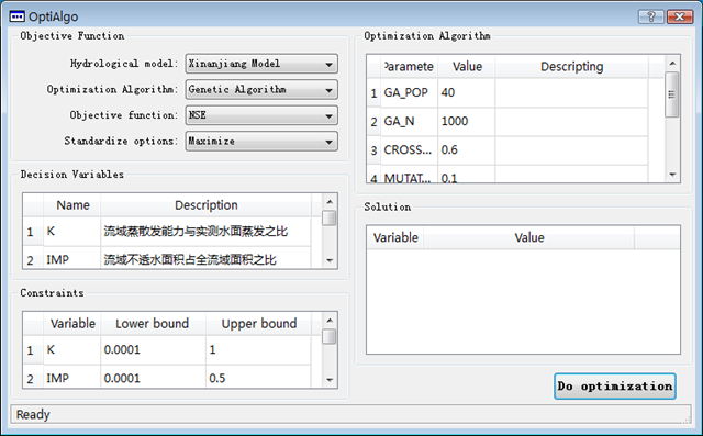
基于Qt实现的优法算法工具包
罐中罐——一种保鲜方法
A Lab for using the PIHMgis and PIHM model (II)
Zhuotong Nan (南卓铜, [email protected])
DEM processing
In this part, we will show you how to delineate a watershed with inputs of DEM(Digital elevation model) and outlet location. Watershed delineation is necessary for any distributed hydrologic model. Although hydrologic models use different software to implement the delineation, the underlying idea and steps are generally common.
1. Open PIHMgis by double clicking the PIHMgis_v2.0.0 shortcut created in the previous section.
2. Enable PIHMgis.
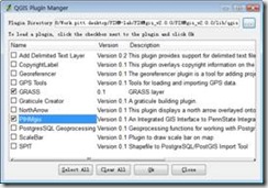
Open Plugin Manager… in the QGIS Plugins menu, tick the PIHMgis item (Figure 3), and press Ok.
Figure 3 QGIS Plugin Manager
Now the PIHMgis toolbar appears as shown in Figure 4.
Figure 4 the PIHMgis v2.0.0 toolbar
3. Load DEM to PIHMgis for displaying.
Layer > Add a Raster Layer…, select lab3.shale.hillsDEMsh_elev.asc.
This DEM file is in ESRI ASCII grid file format. If you have files in ESRI binary grid format which is a proprietary format, you need to convert them to ASCII format by using some ArcInfo command or by some third party tool, such as gdal_translate available from the GDAL website at http://www.gdal.org/.
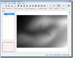
The map view of the DEM file looks like as following (Figure 5),
Figure 5 DEM map view in QGIS
4. Save as a QGIS project. File > Save Project As…, in the Save As dialog, navigate to the directory of lab3.shale.hills, type “sh” for the file name, and then click Save.
Note: During following steps, please save the project frequently. If the project is crashed, you can restore to the previous session by open the project you saved.
5. Fill pits.
Question: Why do we need to fill pits for a DEM file prior to further watershed delineation?
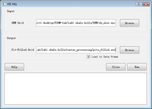
Click the small arrow next to the Raster Processing on the PIHMgis toolbar and then select Fill Pits. This will bring up the Fill Pits dialog (Figure 6).
Figure 6 The Fill Pits interface
Select sh_elev.asc as the input DEM grid and name the output pit-filled grid as “pits_filled.asc” under the “raster_processing” directory as shown in Figure 6. Press Run to start the pit filling process. Click “Close” to dismiss the dialog after the process is done. The pit-filled DEM will automatically be loaded into the QGIS data frame.
6. Calculate flow direction and flow accumulation.
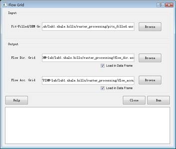
Use the command Raster_Processing > Flow Grid to open the Flow Grid window (Figure 7).
Set pits_filled.asc as the input; flow_dir.asc and flow_accu as the output flow direction grid and flow accumulation grid respectively, also under the raster_processing folder.
Click Run to start the processing. After done, click Close.
Figure 7 Flow Grid
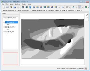
Both flow_accu and flow_dir are shown in the QGIS map view (Figure 8).
Note: the direction codes are following: 1 – east, 2 – North east, 3 – North, 4 – North west, 5 -West, 6 – South west, 7 – South, 8 – South east.
Figure 8 Flow direction generated by PIHMgis
Tip: Within the QGIS framework, visibility of a GIS layer can be switched using the table of contents on left.
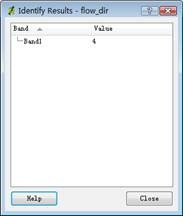
Tip: The identify tool ![]() can be used to identify features by clicking on them in the right map view panel. For example, click on the flow_dir item in the table of contents to make it selected, and then use the identify tool to click over the map view, the Identify Results dialog will pop up and show the value of the clicked feature (Figure 9), here, value of 4 means the point of interest has a flow direction towards north west.
can be used to identify features by clicking on them in the right map view panel. For example, click on the flow_dir item in the table of contents to make it selected, and then use the identify tool to click over the map view, the Identify Results dialog will pop up and show the value of the clicked feature (Figure 9), here, value of 4 means the point of interest has a flow direction towards north west.
Figure 9 Identify results
7. Generate stream grid
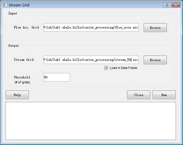
Select Raster Processing > Stream Grid to make the Stream Grid dialog visible, set the flow accumulation grid generated in previous step, i.e., flow_accu.asc, as the input grid, and then set output stream grid to stream_800.asc with a threshold value of 800 (number of grids). Press Run to generate stream grid (Figure 10).
Figure 10 Generate stream grid with a threshold value of 50.
Don’t close the Stream Grid window. Set thresholds to 300 and 800 respectively to compare the resulting stream grids (stream_300 and stream_800 accordingly, Figure 11) and run again.
Figure 11 The generated stream grids with thresholds set to 50, 300 and 800. (left: 50, middle: 300, right: 800)
Close the Stream Grid dialogue by clicking on the Close button.
Question: How to determine an appropriate threshold for a watershed of interest?
8. Generate the stream order grid (known as Link Grid in PIHMgis)
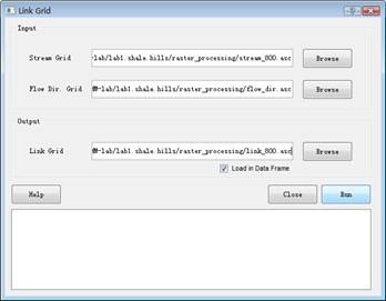
Select Raster Processing > Link Grid to pop up the configure interface (Figure 12). Select stream_800.asc as the input stream grid and flow_dir.asc as the input flow direction grid, and set the output link grid name to link_800.asc (saving to the same raster_processing folder). Click Run to begin processing. After done, the link grid will be shown on the map view panel if the Load in Data Frame option is checked.
Figure 12 Generate a stream order grid
9. Create a vector file of stream network
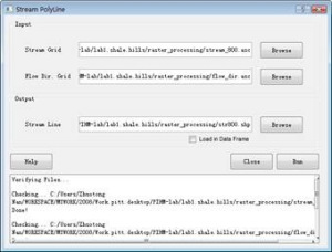
Select Raster Processing > Stream PolyLine to make the interface appear (Figure 13). Set inputs with stream_800.asc and flow_dir.asc generated by previous steps and set the name of the output stream polyline file to str800.shp. Click Run to process it after parameters are specified.
Figure 13 Create a vectorized stream network
10. Generate catchment grid and its corresponding vector file
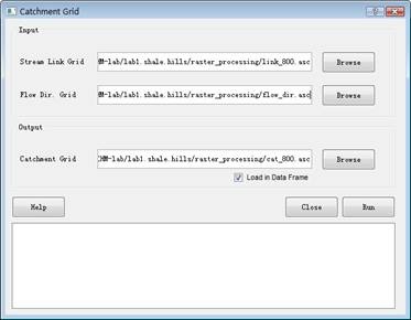
Select Raster Processing > Catchment Grid to bring up the catchment grid generation interface (Figure 14). Set Stream Link Grid to link_800.asc, Flow Dir. Grid to flow_dir.asc, and output Catchment Grid to “cat_800.asc”. Both input and output files are located in the raster_processing directory.
Click Run to start calculating the catchment grid. Click Close to dismiss the dialog.
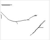
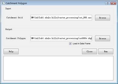
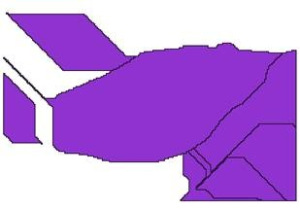
Select Raster Processing > Catchment Polygon to display the interface for converting grid catchment file to vector (Figure 15). Set input to cat_800.asc and output to cat800v.shp. Run to start the processing and Close to dismiss the window. The resulting catchment polygons are shown on Figure 16. Note: the color to render the polygons might not be same as that on the Figure 16, as it is determined by QGIS automatically.
Figure 14 Catchment grid generation interface
Figure 15 Convert catchment grid to vector
Figure 16 Resulting catchment polygons
11. Extract the watershed boundary of interest
The current PIHMgis version 2.0 does not provide such a function to clip the watershed boundary under study and stream network within it. We need to do this by help of other GIS software such as ESRI ArcInfo, or by using QGIS editing capability demonstrated below. In the future version of PIHMgis, this functionality will be implemented. To determine the boundary of a watershed, the outlet location should also be specified.
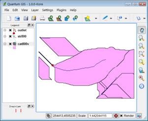
Open QGIS 1.0, load cat800v.shp and str800.shp generated in previous steps to the data frame using Layer > Add Vector Layer…, and then load outlet.shp, which contains outlet location. The view now looks like Figure 17.
Figure 17 QGIS 1.0 with stream network, catchment polygons and outlet layers loaded
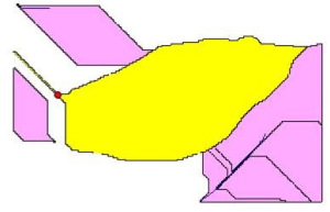
Click on cat800v within the table of contents to make it the current layer. Use “Select Features” tool (Figure 18) to select the watershed polygon of interest (Figure 19). The selected polygon is now in yellow. If the tool is invisible, just drag the toolbar to a new place to make fully appeared.
Students are advised to have a look at all built-in toolbars, making them familiar with all those often-use tools.
Figure 18 The Attributes toolbar
Figure 19 Select the watershed of interest
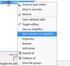
Right click the cat800v item and select “Save selection as shapefile…” to save the selected polygon (Figure 20) to a new shapefile, here, “cat800v_sel.shp”, under the “raster_processing” folder. If you are required to select a project, click OK to use the default one.
Note: The default project probably is not correct, but does not matter with following operations. You can change the project in a layer’s property window later.
Figure 20 Save selection as a new shapefile
Similarly, select the corresponding stream from str800 and save as a new shapefile “str800_sel.shp” (Figure 21), also into the “raster_processing” folder. If you are required to select a project, click OK to use the default one.
Figure 21 Select the corresponding stream, shown in yellow.
Load str800_sel and cat800v_sel into the QGIS map view. Drag layers up or down to rearrange layers’ visibility. Uncheck str800 and cat800v to hide them. Now the map view looks like Figure 22.
Figure 22 Load str800_sel and cat800v_sel and hide str800 and cat800v
Make str800_sel disappear. Select “cat800v_sel” layer, and use “zoom in” tool (the one w/ magnifier icon and a plus symbol shown in Figure 23) to enlarge the area near the outlet. Click “Toggle editing” tool (the one w/ pen icon shown in Figure 23) to make the current layer editable (Figure 23). Now the other tools on the Digitizing toolbar are also available when the layer enters into edit mode. The tools may be hidden, in this case drag toolbars to a blank place to make all tools shown.
Figure 23 cat800v_sel in edit mode
Click the Split Features tool. Draw a curve to cross the outlet so as to split the whole polygon. Right click to finalize the curve; the Split Features will then split the polygon. Click the “Toggle editing” again to make the layer back in the normal view mode. Make sure saving it if you are asked to save the features.
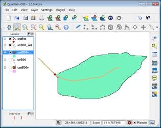
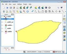
Use “Select Features” tool to select the large polygon right to the outlet. If the previous operation has been done successfully, only the large part will be selected and the upper left part remains unselected. Save the selected polygon to a new shapefile named “cat800v_clip.shp”. Load cat800v_clip to the map view. It now looks like as shown on Figure 24.
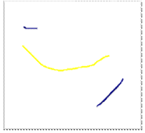
Figure 24 Clipped watershed boundary
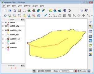
Similarly, we also split the str800_sel.shp. Make it visible and editable, draw a curve to split it across the outlet, save the operation, and then export the desirable line (on the right) to a new shapefile, “str800_clip.shp”. (Figure 25)
Figure 25 Clipped stream network
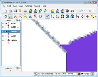
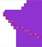
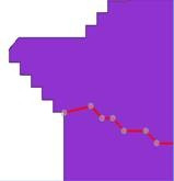
Zoom in the outlet area, and carefully edit the stream polyline making its end node locate on the watershed edge. However no necessary exact alignment is needed. Tools for vertex editing are shown in Figure 26. The final stream line looks like as in the Figure 27. Save the stream file after done.
Figure 26 vertex editing tools. Left: move vertex; middle: add vertex; right: remove vertex
Figure 27 Align the end node of stream line to the boundary. Left: original; right: edited
Close QGIS 1.0.
小熊挣了好多钱
这两天给家里的电话总是不通,先是朵朵妈妈手机被偷,再是欠费停机。今天再试了一下,却意外惊喜的发现通了。她们正坐在机场到兰州的出租车上。没跟小赵说两句,朵朵就说她要发言。接过后,她说,爸爸,小熊挣了好多钱,回来小熊将钱给你呀。她的最喜欢的玩具小熊吗?不是很明白她的意思。当我问的时候,朵朵抗议说信号不好,不跟我讲了。她妈接上后,说朵朵说要改名了,不叫朵朵叫小熊了,原因是她感觉小熊好可爱。这趟回老家的时候,可能大人给了她不少压岁钱,说要给爸爸。原因是爸爸没钱,妈妈有很多钱,最重要的是,爸爸会用钱给朵朵买糖吃,总归还是为好她自己着想呢。
Talking about 也说内存
这是似是而非而且荒谬的结论,而且同样极端了。
不管内存有多少G了,相比硬盘比还是很小。所以在完成任务目的,保证用户可接受的速度下,优化内存当然是性能的一个重要指标了。写程序的时候永远无法知道运行这个程序时的计算机情况,当然能节省则要节省了,一般程序很少去智能调整自己内存占有,优化程序的内存使用是现代操作系统的重要任务。节省越多的内存,意味着可以同时并存更多的程序,这是为用户负责的一种表现。
举个极端的例子,程序A完成既定任务用1M内存在多数配置机器上可以比较流畅的运行了,这时目标机器上还有2G的内存可用,OK,照“充分利用内存”的说法,意思就是最好将2G都“充分”用起来,OK,程序A充分用了1G的内存(嗯,程序A load了除了必要的执行代码和必要的数据,将潜在操作有可能用到的文件也顺便load进来了,这样对1%的用户来讲可能提升了 0.0001%的速度,这符合“充分使用内存”吧),目标机器上还有1G剩余的(幸好不是只剩1K内存了)。问题是,1M内存使用的时候速度已经不错了,用1G内存提升的速度并不明显。但为了这一点速度上的优化被你“充分”占了1G的内存。目标机器接下去还要再运行一个专业软件,而这个软件需要load一个1G的数据进内存,my god,stupid的操作系统接下去做的事情就能让你发疯。就是因为程序A根本无法预料到用户机器的情况,从而根本无法做到“充分”利用。你能做的就是,保证性能的前提下,尽量优化内存使用,尤其对于大型程序来讲。
让程序去根据内存可获取情况自动调整自己的内存占有情况? 当然可以,但有这时间,不如去开发更多的大家需要的功能。而且操作系统已经具备多数情况下行之有效的算法去优化这些程序的内存使用,尽管有时候很stupid。
“所以,最终结论是”,即使“在内存使用不超出最大物理内存的情况下,比如在大内存的PC机上(大内存指内存接近或超过4G—4G是32位地址的范围,比如2G或3G或8G)”,也不能为了一点点的速度提升去“充分”利用内存。“内存多使用并不是什么错,不要再把内存使用多少作为性能标准了”,这是对的,但“我们追求的性能”不仅仅是“速度”,还有对用户负责的一种态度。——除非,增加内存使用可以明显提高各方面的性能,那又是另一个story了。
恭喜cathy拿到诸多好大学的offers
我早说过,这次肯定会挑花眼的。看来我的感觉很正确。记得请客吃饭。
Documentary film on the global warming issue presented by former US vice president Gore
A friend recommended a *documentary* movie presented by the former US vice president Gore on the topic of global warming. It takes totally approx. 1hr30 min in length. I would like to share it with all of you. Very good movie worthy all of you have a look at it.
BTW, the movie is presented in English, but also with a good Chinese translation on the screen.
Following please find the links,
Part 1. http://www.tudou.com/programs/view/HoJM-FFBL5g/
Part 2. http://www.tudou.com/programs/view/9Fxft4eiyN8/
Part 3. http://www.tudou.com/programs/view/lZEjFpbrf3Y/
Part 4 : http://www.tudou.com/programs/view/LdBZIFXborQ/
In the Part 3, we also can see Prof Yao Tangong who introduced the facing challenges to Gore.
Latest Flash player should be installed in order to see the movie online.


