Tag Archives: arcgis

在Arcgis 10.2里对raster 做reclassify 的时候,提示字段乱码无法成功

事件重现:

一个dem raster数据,对其做spatial analyst > neighborhood > focus statistic,取值最大值,然后进行 reclass > reclassify。focus 能正常生成,但在reclassify 的时候提示:

The name of the Field is invalid: valid names may contain letters, numbers or underscores.

里面的大概story 是这样(猜的),dem 是中文平台上生成,采用的编码大概是 gbk 之类的,做focus 时会生成一些dbf 字段,于是也采用 gbk,但reclassify 大概采用utf 去读gbk,于是不识别。

我采用的方法是:

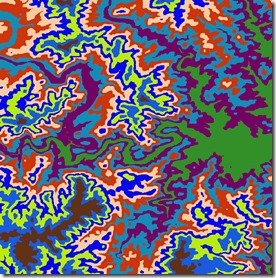
新建personal geodatabase,将 dem import 进这个gdb,然后做 focus & reclassify。

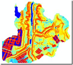
最后的图蛮漂亮的。

reclass-result

Arcinfo Generate 格式转Shapefile 的方法

Arc/Info Generate 格式已经有点历史,现在版本的ArcMap 都不能直接支持对该格式的读取。但由于Generate 格式对矢量数据模型的表达十分简明,在教学中仍然还广泛提及。为了看看Generate 文件的地图效果,需要把该格式转为Shapefile 等格式,才能在ArcMap 中显示。

第一种转换的方法是使用ArcGIS 的Data Interoperability 模块

ArcGIS Desktop 里需要安装 Data Interoperability 模块,在ArcMap Extension 里将该模块打勾,然后通过 ArcToolbox 下的 Data Interoperability Tools 里的Quick Import 将Generate 文件导入到Shapefile 或者 Geodatabase。

Data Interoperability 实际上是调用了内置的FME Reader 来实现格式互转,ArcInfo Generate 的短名是ARCGEN。如果Generate 文件后缀是.gen,在import时可以被自动识别;如果不是.gen,则需要手动设置输入格式是ARCGEN。

第二种转换方法是使用第三方工具 gen2shp (提供可执行文件下载)

Continue reading

关于Personal geodatabase拷贝给他人用的问题

Personal geodatabase是利用Access数据库进行ESRI Geodatabase数据模型的物理存储。以前是不支持栅格数据的存储,矢量数据都放在一个.mdb里,很方便将这个mdb文件拷贝给别人。当然Personal GDB只支持Windows,但因为国人多数只用Win平台,一般不是大问题。

任一种GDB拷贝给别人的时候,都会关注版本的问题,如果自己的ArcGIS版本太高,一般默认的是GDB版本也高,他人如果是使用较低版本的ArcGIS是无法打开高版本的GDB的,所以最好将GDB版本降到9.x再给别人。

Personal GDB现在是支持栅格,这时,应该拷贝给别人的文件除了.mdb外,还要包括一个xxx.idb的文件夹,这里xxx是GDB的名字,注意这是一个文件夹的名字。如果忘了拷贝这个idb文件夹,他人收到是无法打开其中的栅格文件,但其中的矢量文件是可用的。最近我给他们拷贝时就发生这个的问题。

事实上,这时候Personal GDB就失去了以往单一文件便于传递的优势了,我建议不如使用File geodatabase这一不受平台限制的GDB格式。

ArcGIS 10文档有时候不准确

在Arcmap 10的Python Window里执行 MosaicToNewRaster_management时,按其文档给出的例子对应修改各个参数,发现总是提示Cannot set input into parameter coordinate_system_for_the_raster错误,即投影文件参数没有设对。

ArcGIS 10文档里的例子:
arcpy.MosaicToNewRaster_management(“land1.tif;land2.tif”, “landnew.tif”, “World_Mercator.prj”, “8_BIT_UNSIGNED”,  “40”, “1”, “LAST”,”FIRST”)

函数原型:
MosaicToNewRaster_management (input_rasters, output_location, raster_dataset_name_with_extension, {coordinate_system_for_the_raster}, {Pixel_type}, {cellsize}, Number_of_bands, {mosaic_method}, {mosaic_colormap_mode})

仔细对照其参数列表,发现参数列表里比例子多了一项,即在投影参数前有两项,一项是输出位置,一项是输出文件名,而不是列子里只有一项。修正后问题仍然存在。

不过现在的问题是找不到投影文件.prj,将之扩展为绝对路径即可以执行。

我猜ArcGIS文档里一些例子是以前版本的,在新版本里参数发现了变化,但例子没有及时更新过来。所以大家在使用时,还是不能尽相信例子,当发现问题的时候,对照函数原型会更靠谱。

Workflow of Preparing Stream Data for DHSVM

Workflow of Preparing Stream Data for DHSVM

Zhuotong Nan (南卓铜, [email protected])

Preparing stream data for DHSVM is very complicated. Many AML scripts as well as Java are involved. Through the example showed below, I want to examine what the preparation really does and what happens behind the scripts. The scripts need ArcGIS workstation, which is not commonly installed. Thus I wrote this article, in the hope that without installation of ArcGIS workstation, you can see clearly the processes and if you want you can re-implement it with other languages.

I created a folder named “highplandpark” on the desktop, whose actual path is c:usersnztdesktophighlandpark. The contents in this folder include,

  • Arcscripts, directory, the aml scripts copied from DHSVM.
  • Programs, directory, the java codes copied from DHSVM
  • Dembuilding_my.asc, file, dem file
  • Mask.asc, file, the mask file for the area of interest

Those files can be found here.

In order to repeat the following steps, ArcGIS Desktop and Workstation, Java Runtime Environment JRE, shall be installed as prerequisites. I used version 10.0 for both ArcGIS Desktop and Workstation and JRE 7. My OS is Windows 7 x64.

image
Generated soil depth grid

Read the 18-page full document, pdf (478KB)

Two attached files

用ArcGIS读取GIMMS AVHRR NDVI 3g 数据

用ArcGIS读取GIMMS AVHRR NDVI 3g 数据

[email protected]

这个第三代NDVI数据,文件名类似于geo82dec15a.n07-VI3g ,增加.bsq扩展名,比如geo82dec15a.n07-VI3g.bsq。

然后建立一新文件,文件名与ndvi文件名一致(不包括.bsq),扩展名为 .hdr,如geo82dec15a.n07-VI3g.hdr。把此.hdr与nvdi文件放在一起。.hdr是个文本文件,内容包括:

nrows 4320

ncols 2160

nbands 1

nbits 16

pixeltype SIGNEDINT

byteorder M

layout bsq

在arcgis里就可以以栅格的形式打开。不过遗憾的是,由于ndvi 3G文件好像写数据的次序与arcgis不一样,所以读出来是倒置的。

在ArcGIS里做一个栅格transpose rotate,就是正确的图像。然后增加正确的坐标信息,在正确位置下,坐标信息如下:

upper-left-lat: 90.0-1/24

    upper-left-lon: -180.0+1/24

    lower-right-lat: -90.0+1/24

    lower-right-lon: 180.0-1/24

Geographic Lat/Lon

    pixel-size: 1/12=0.0833 degrees

因ndvi3g读过来的数据中包括flag信息。用raster algebra计算ndvi时,用以下公式,

ndvi = rounddown(ndvi3g / 10) / 1000

标志flag

flagW = ndvi3g – rounddown(ndvi3g / 10) * 10 + 1

(注意栅格运算时,操作符之间是必要有空格的。)

标志含义

The meaning of the FLAG:

    FLAG = 7 (missing data)

    FLAG = 6 (NDVI retrieved from average seasonal profile, possibly snow)

    FLAG = 5 (NDVI retrieved from average seasonal profile)

    FLAG = 4 (NDVI retrieved from spline interpolation, possibly snow)

    FLAG = 3 (NDVI retrieved from spline interpolation)

    FLAG = 2 (Good value)

    FLAG = 1 (Good value)

由于Arcgis需要多个操作,建议用Matlab或别的编程语言自己写点代码来处理。

arcgis的中文路径问题

1. arcmap显示地图一块是fully 兼容中文路径的。但发现在执行一些分析时,仍受影响。比如当执行 spatial analyst里的 extract values to points,会提示错误。这时把数据文件都移动一个无中文路径的目录下是可以正常执行的。

2. arcmap 10里无法计算 solar radiation,更新到sp4 可以正常计算。

3. 另外,fyi,那个cracked arcgis 10 license manager在 sp4是可以用的。不过当安装完sp4,需要重新安装一下那个 crack。

image

ArcGIS 10 license

Arcgis Desktop 10安装后,D版盘里还有个Crack_LM_ArcGIS10目录,里面有Crack_LM程序,运行后生成c:Cracked License Manager 10目录,以及将一个afcore库copy进arcgis相应的位置。不必安装arcgis10自带的License Manager。

注意,除了lmgrd.exe要解除firewall,arcgis.exe也要解除,否则不能使用。

破解License的目录(c:Cracked License Manager 10),不能改名。如果不中意此名,一定要修改的话(以修改成ArcGIS License Manager 10为例),可以用以下方法:

1. 任务管理器里找到lmgrd.exe, 结束之。arcgis.exe因为是lmgrd.exe调用,会自动结束。

2. 在资源管理器里,将Cracked License Manager 10 修改为ArcGIS License Manager 10。

3. 用记事本打开此目录下的start_lic_mgr_invisible.vbs,将其中的Cracked License Manager 10 改为ArcGIS License Manager 10。保存关闭。

4. 用记事本打开start_server_license.bat,将Cracked License Manager 10 改为ArcGIS License Manager 10。保存关闭。

5. 点击,开始 > ArcGIS License Manager 10 CRACKED > ArcGIS License Manager 10 CRACKED 会提示 lmgrd.exe 和 arcgis.exe 的security alert,全部 allow access。

6. 打开 arcmap 10 测试 是否正常运行。

7. 到防火墙设置里,允许通过列表,去掉 原先在 cracked … 目录下的arcgis.exe 和 lmgrd.exe(列表名叫Acresso Software Inc.)。

Done!

Using ArcGIS to prepare Sub catchment file for TopMODEL

Zhuotong Nan ([email protected]), CAREERI/CAS

TopMODEL is a conceptual hydrological model which was initially released in 1979 but is still widely used today especially in a watershed simulation with sparse observations.  TopMODEL uses topographic index (TI) to calculate water flow. There are already some tools developed for TI computation. Here I want to present a method using ArcGIS.

There is a similar work at http://soilandwater.bee.cornell.edu/Courses/GIS/TI.ppt. What I will present will be more than it.

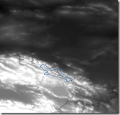
1. We have  a DEM which is large enough to cover our study area. The DEM “Heihe_SRTM.img” is subset from the SRTM 90m data which is in lat/lon coordinates (WGS84).
image

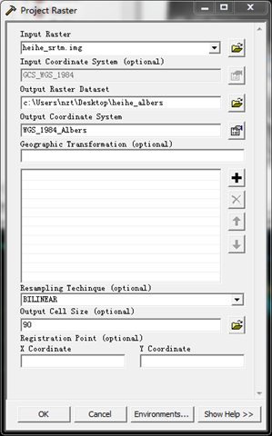
2. Open ArcToolbox, go to Data Management Tools > Projections and Transformations > Raster > Project Raster.
image

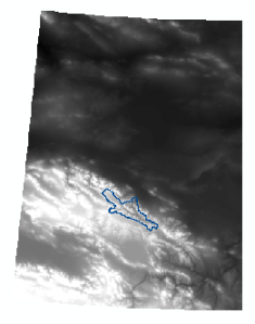
Here use bilinear to interpolate the input raster to a 90m resolution grid in the Albers equal area projection.  The resulted raster is “heihe_albers”.
image 

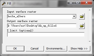
3. In ArcToolbox, Spatial Analyst Tools > Hydrology > Fill, to fill up the possible sinks, resulting “hh_up_filled”.
image

4. In ArcToolbox, go to Data Management Tools >Raster > Raster Processing > Clip, to make the filled DEM smaller, because the next steps are very computation intensive. “dem_up_fil” is created.
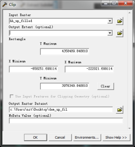
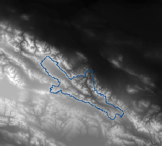
image image

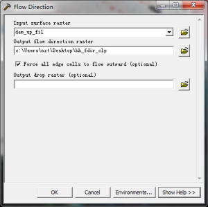
5. Hydrology > Flow direction. Note, use the filled DEM. flow direction file is “hh_fdir_clp”.
image

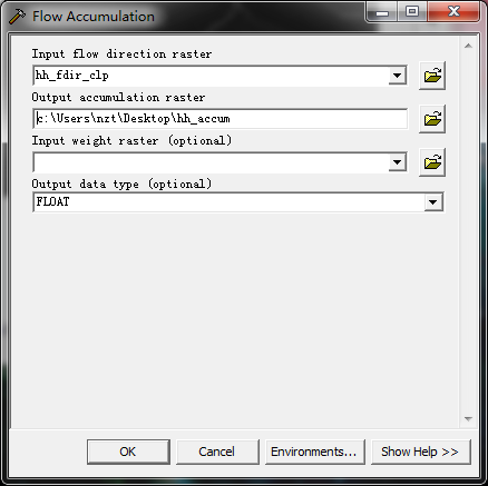
6. Hydrology > Flow Accumulation to compute “hh_accum”
image

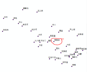
7. open hydrosta.shp. this is a hydrological station location shapefile. We use the red line surrounded site as the watershed outlet.
image

8. use the “select feature” to select the desired site

image image

9. export to a separate file. the exported ylx.shp now is in same projection as hydrosta.shp which is lat/lon.
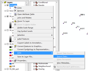
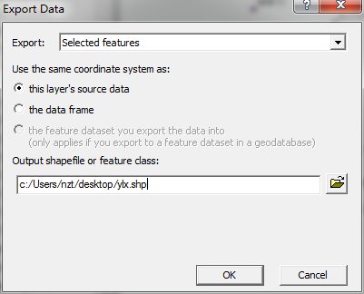
image image

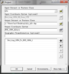
10. Data Management Tools > Projections and Transformations > Feature > Project. save as “ylx_alb.shp”.
image

the output coordinates can be imported from the heihe_albers raster.

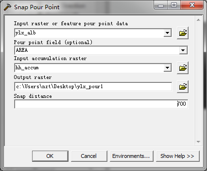
11. Hydrology > Snap Pour point. Carefully select the snap distance which is in map units. The result is “ylx_pour1” grid.
image

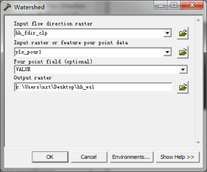
12. Hydrology > Watershed to delineate the watershed. Now we have “hh_ws1”.
image

13. ArcToolbox > Conversion Tools > Raster to Polygon to create “hhupws.shp”
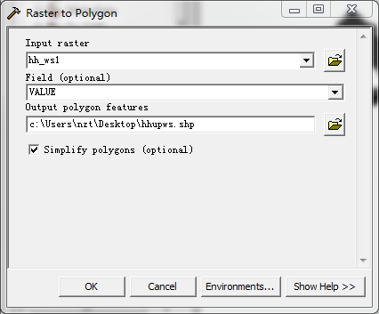
image image

14. Open Spatial analyst toolbar (right click on the blank space of menu bar, select Spatial Analyst), set Spatial Analyst > Options > Analysis mask to hhupws (the watershed boundary polygon)
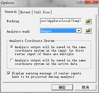
image

15. Spatial Analyst > Raster Calculator, double click hh_fdir_clp, and then click Evaluate. This will make the hh_fdir_clp masked by the watershed boundary.
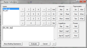
image

Make the generated Calculation layer permanent (right click the item in the TOC, Data > Make Permanent…). Save as “hh_fdir_up1”.

Do same to dem_up_fil; dem is clipped to “dem_upstr1”.

Do same to hh_accum to generate “hh_accum_clp”
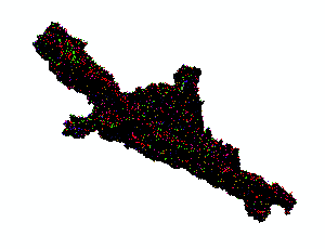
image image image
hh_fdir_up1 (left), dem_upstr1 (middle) and hh_accum_clp (right)

16. Hydrology > Flow Length
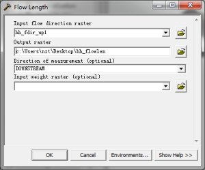
image

the flow length raster “hh_flowlen” is used to calculate channel levels in the SUBCAT file.

17. Spatial Analyst > surface analysis > Slope
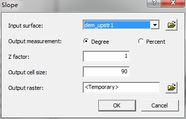
image

save the slope file as “Slope_filldem”

18. Spatial Analyst > Raster Calculator
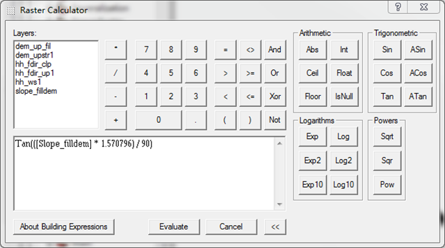
image

use “Tan(([Slope_filldem] * 1.570796) / 90) ” to calculate tangent of slope radians

save to “tan_slope1”

19. Same in Raster Calculator

Calculate TI by typing “Ln((([[hh_accum_clp]] + 1) * 90) / [[slope_filldem]] )”
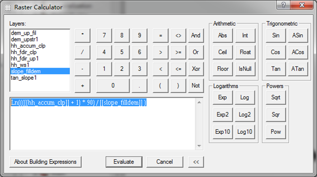
image

save to “ti1”

Now we have data ready. What we do next is to classify data and make data formatted to fit what Topmodel requires.

20. Select ti1, then click Spatial Analyst > Reclassify … In the window, click Classify, select Equal Interval as the method, set 29 as the classes, click Ok to accept it. Other classification methods also can be used for your cases. You also can set more classes. but keep in mind that the TopModel version might be have limitation on classes.
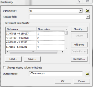
image

click “Save…” , save the classification schema to “ti_table” as info table

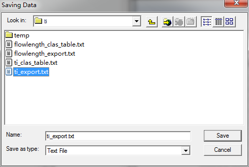
Click ok to classify the continuous TI grid. a new layer “Reclass of ti1” is added to TOC. select it and right click to bring up the context menu. Open Attribute Table, and then Options > Export all records to “ti_export.txt”.
image

Note, the Save as type should be selected as “Text File”. It might not work if you only specify an “.txt” extension.

Do same to the hh_flowlen. classify it to 9 classes. and export the data to “flowlen_export.txt” in a text format. The classification schema is saved to “flowlen_table”.

21. In ArcGIS, click Add data to adding flowlen_table and ti_table to the ArcGIS session.  Right click on each item, open the table, and export all data to text files, here, “flowlength_clas_table.txt” and “ti_clas_table.txt”, respectively.

image

22. Open Excel. drag “flowlength_clas_table.txt”, "ti_clas_table.txt”, "ti_export.txt”, and “flowlen_export.txt” to Excel.

In each Excel workbook, select the first column, click “Text to Columns” in the data tab of Excel 2007. in the earlier version, there is also similar commands.

select comma as the delimiter, click finish.

Copy “From_”, “To_”, “Out” columns in class schema files, append to ti and flowlen export data workbooks respectively. This step is to combine the schema to actual data. after appending, close the two class table files (“flowlength_clas_table.txt”, "ti_clas_table.txt”) without saving changes. Now we have something like that,
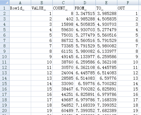
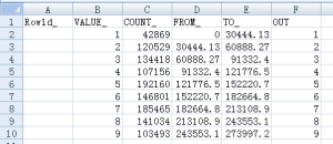
image image
The combined ti_export.txt workbook(left) and the combined flowlen_export.txt workbook (right)

23. In the ti_export.txt workbook, select the “OUT” cell, click reverse order command image .

Right to the “OUT” column, add “Area”, and then “TI”. 

In the cell below the title “Area”, type: =c2/sum($c$2:$c$30).  this will calculate the fractional area. Note, $c$30 indicates the last low of the data. You might change it accordingly when you have different classes. Copy this cell to propagate through the Area column.

In the cell below the title “TI”, type: =D2. Copy this cell to propagate through the Area column.

Insert a new row right below the header row where we set area to 0, and ti to “=E3” (the largest TI). like below in this time,

image

Save the result to a new Excel file, say, “ti_ready.xlsx”.

24. In the flowlen_export.txt workbook, right to the “OUT” col, add “area”, “accum_area”, and “dis” in the next two cells.

use “=C2/SUM($C$2:$C$10)” to calculate the area column; note, $c$10 is the last data line. change it accordingly.

use “=SUM($G$2:G2)” to calculate accumulative area for the accum_area column;

use “=e2” to calculate the dis column.

copy those formula to other rows.

insert a new line immediately below the header line. type 0 and 0 for accu_area and dis.  if this is a subcatchment, set the distance from the outlet of the entire catchment to dis here.

looks like as below,

image

save the excel to “flowlen_ready.xlsx”

close ti_export.txt and flowlen_export.txt, no need to save changes.

Note, we do not need to reversely sorting data which is different from the ti case described above.

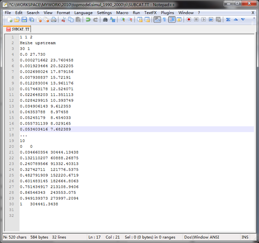
25. copy “area” and “ti” in the ti_ready.xlsx (without header) to the proper section of the SUBCAT file.

copy “accum_area” and “dis” in the flowlen_ready.xlsx (without header) to the proper section of the SUBCAT file.

in this case, the total ti increments are 30; the total channel levels are 10. looks as below,
image

For the demonstration purpose, we abbreviate 30 ti increments.
Out of memory problem

两个目录下有66K多个文件,需要运行Kappa进行计算比较。作了一个批处理,

for %%f in (C:nan_wkspmetric_analysis_radar_nldasdatanwbi_deg8_selradar_clas*.asc) DO (
kappa %%f C:nan_wkspmetric_analysis_radar_nldasdatanwbi_deg8_selnldas_combo_clasl%%~nf.asc -k:C:nan_wkspmetric_analysis_radar_nldaskappakappa.txt)

在执行到1万个的时候,提示 Not enough storage is available to process this command,以及 out of memory,退出!不知道是什么原因。起先以为是Kappa代码有问题,但理论上讲,代码是用托管模式写的,正常退出时dotnet会负责回收的。Kappa代码里连接了ArcGIS的相关代码,这部分是非托管的,有可能是异常引起非托管资源被占用,从而积累导致问题。

后来在网上找了一下,在微软KB里有类似的描述,http://support.microsoft.com/kb/126962,建议修改注册表,增加shared memory。

但终因为不知道改成多少合适,而且改Kappa代码也很容易,决定不采用这种方法(workaround)。用c#写小段代码,实现批处理,寄希望于通过托管系统自身的回收机制,能解决out of memory的问题。代码十分简单。

using System;
using System.Collections.Generic;
using System.Linq;
using System.Text;
using System.IO;
using System.Diagnostics;

namespace Kappa_bat
{
    class Program
    {
        static void Main(string[] args)
        {
            string nldas_dir = @"C:nan_wkspmetric_analysis_radar_nldasdatanwbi_deg8_selnldas_combo_clas";
            string radar_dir = @"C:nan_wkspmetric_analysis_radar_nldasdatanwbi_deg8_selradar_clas";
            string out_dir = @"C:nan_wkspmetric_analysis_radar_nldaskappa";

            string kappa_file = Path.Combine(out_dir, "kappa.txt");
            string log_file = Path.Combine(out_dir, "logfile.txt");

            string[] radarfiles = Directory.GetFiles(radar_dir, "*.asc");
            foreach (string f in radarfiles)
            {
                Process proc = new Process();
                proc.StartInfo.FileName = "kappa.exe";
                string fn = Path.GetFileName(f);
                string nldas_fn = Path.Combine(nldas_dir, "l" + fn);
                proc.StartInfo.Arguments = nldas_fn + " "+ f+ " -l:"+log_file+" -k:"+kappa_file ;
                proc.StartInfo.UseShellExecute = false;
                proc.StartInfo.RedirectStandardOutput = true;
                proc.Start();
                proc.WaitForExit();
                Console.WriteLine(fn);
            }
            Console.WriteLine("Done.");
        }
    }
}