一种简单有效的MODIS LST内插方法
Zhuotong Nan ([email protected], 南卓铜)
本软件实现了一种新的基于相似性原理的MODIS陆表温度(LST)的插值方法。这种LST数据空间插值方法利用具有相似温度变化特征的已知LST像元集合推算缺失的LST。在青藏高原的案例表明传统的地统计方法基本无法处理大范围连续的数据丢失(比如因为云),而本方法明显优于传统方法,可能较合理的得到缺失LST。此方法尤其适用于大范围山地区域。
This tool implements a new interpolation method for MODIS land surface temperature (LST) following the theory of similarity. It estimates the missing LST pixels by known LST pixel sets which bear similar characteristics of LST variation as the missing pixels. A case study on the Qinghai Tibet plateau has already been carried out, showing its obvious advantages over the traditional geostatistic methods, the latter was unable to do with a large area and temporally continuous data missing situations. This approach is especially good for a study area with a large area and mountainous terrain.
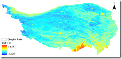
fig 1a, with this approach
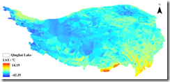
fig 1b, with Kriging
1. Mosaic and resample
1.1 Put your raw HDF files in qz.lst.hdf.2005. The raw HDF files may have a name convention as below,
MOD11A1.A2004001.h23v05.004.2004004053641.hdf MOD11A1.A2004001.h24v05.004.2004004052114.hdf MOD11A1.A2004001.h24v06.004.2004004053201.hdf MOD11A1.A2004001.h25v05.004.2004004052024.hdf MOD11A1.A2004001.h25v06.004.2004004051831.hdf MOD11A1.A2004001.h26v05.004.2004004045717.hdf MOD11A1.A2004001.h26v06.004.2004004051758.hdf MOD11A1.A2004001.h27v05.004.2004004045634.hdf MOD11A1.A2004001.h27v06.004.2004004045506.hdf
In this case, the study area has covered nine scenes. Put them together, the tools will take care of the processing.
1.2 Create a folder qz.tif.2005 and a folder temp. The qz.tif.2005 is the location the output will be put in and the temp is the location for storing temporary files generated during the process.
1.3 Open modislst2tif_bat_config.txt under the process.codes folder. The file may look like as following,
startday= 2005171
endday=2005365
datafilepath = “../qz.lst.hdf.2005”
temppath = “../temp”
tifpath = “../qz.tif.2005”
removetemp = false
where, startday and endday indicate the starting day and the end day of the raw LST HDF files. The datafilepath specifies the location where the raw HDF files are in. temppath is a location for storing temporary files produced during the process. tifpath is the target location the generated tiff files are put. if removetemp is false, the temp files will not removed after the completion of this process, which is generally useful for debugging purpose. otherwise, with the option of true, the temp files will be removed after completion.
Change it if you use different paths.
1.4 Open LST.prm in the process.codes.folder with any text editor. If you are working with a different spatial extent, change SPATIAL_SUBSET_UL_CORNER and SPATIAL_SUBSET_LR_CORNER accordingly. UL and LR indicate upper left and lower right. They are in latitude and longitude. DO NOT CHANGE OTHER SETTINGS.
1.5 Open your command window, change to the process.codes folder. For example, Press win+R and type cmd, type “cd your/path/to/process.codes”. Note, replace your/path/to/process.codes with your real path.
Type modislst2tif_bat to execute the scripts, which will generate TIFF files as per your settings in modislst2tif_bat_config.txt.
After this step, we have mosaiced tif files, including day, night, qc for both in the folder of qz.tif.2005.
2. clip the tif files to the study area
2.1 Crate a folder named qz.tif.2005.clp.
2.2 Open clp_qtp_bat.py under process.codes/clp_bat. This python code needs the support of ArcGIS 10.0. You may change the settings according to your real needs. After saving your changes and double click the script to run.
The output will be in the folder, qz.tif.2005.clp. You can change the path in the python file.
In this example, a file named qtpbnd_geo_10.shp under the qtp.shape folder defines the clipping boundary. If you are working with other area, put your boundary shapefile on a folder, and then make changes to the variable clpshapedir and the file name in the following line of code. For example, if you current clipping shapefile is xxxx.shp, just replace it as,
#bnd shape
qtpbnd_geo_10_shp = os.path.abspath(os.path.join(clpshapedir,”xxxx.shp”))
You many also want to change the extent of the xxxx.shp, change the following codes to a proper extent.
# Process: Clip…
gp.Clip_management(raster, “73.4191055297854 25.9992794598377 104.428881201583 39.8155412791515”,
Output_Raster_Dataset, qtpbnd_geo_10_shp, “”, “ClippingGeometry”)
3. processing quality control flags
3.1 Create a folder named qz.tif.2005.flg.processed.
3.2 Open the matlab script process_flags.m with Matlab. Pay attention to the variable settings at the top, and make sure they are correct. If you are not with the 2005 data, your LST file naming pattern may not start with “MOD11A1_2005”, change them accordingly to reflect your data.
3.3 Run this script with your matlab. The output will be in qz.tif.2005.flg.processed.
This step will make pixels as missing, if they meet the quality control criteria.
4. Use Excel to determine reference images.
4.1 Locate stat.txt under the qz.tif.2005.flg.processed folder. This file was created in the previous step.
4.2 Import this text to Excel, and split into Excel column by using Tab as separator.
4.3 Determine reference images which have highest percentage of pixels in good quality. The last column indicates the good quality fraction. You may find multiple reference images to represent different season and timing.
For example, in the Tibet case, we divide the whole year into two seasons, warm (days 121-273) and cold (days <121 or > 273). Then we can find four reference images of 2005 to represent day and night images for these two seasons. They are,
cold, day, MOD11A1_2005349.LST_Day_1km.tif, 0.930604881
cold, night, MOD11A1_2005301.LST_Night_1km.tif, 0.932858849
warm, day, MOD11A1_2005251.LST_Day_1km.tif, 0.94265371
warm, night, MOD11A1_2005250.LST_Night_1km.tif, 0.959818432
You should locate the reference images for your case.
4.4 Open interp_ref2.m in the folder process.codes/matlab. Look at the variable settings on the top. Change the ref_fns accordingly to use your reference images names.
If there are more than four reference images, extend ref_fns dimension and then change “for i=1:4” accordingly.
Interpolated reference images are in qz.tif.2005.ref.interp2.
5. Interpolate the LST files.
5.1 This method still needs DEM, slope and aspect. In the Tibet case, they are located in qt.1km.dem folder. Be careful those three tif files should be clipped with the same boundary file such as qtpbnd_geo_10.shp as the LST file did. otherwise, the dimension may be inconsistent during the interpolating process.
5.2 Open the interp_lst3.m under the process.codes/matlab. Pay attention to the path setting on the top of this file and make sure they are correct.
Also look at the file name pattern at the line 26, change it to match your file name pattern if you are with different year.
The output folder is qz.2005.lst.interp.
The codes use distributed computing which can make full use of the multiple CPU. By default, it use 8 CPUs; if your computer have different size of CPUs, change it at the line 94.
For a large area, the computation make take long time. In that case high performance computers are preferred. For smaller area, use of Workstation PC is ok.
If you meet any problem, please feel free to write me via email, in which you well describe the problem. I cannot guarantee I will response immediately, but I will make my time to help you.
Download the tool (27,964KB) / available upon request
MD5 Sum:
75b2377e3fb7c2997784ebe0844c19b8 soft.modis.lst.interp.2014.zip
The readme document (pdf, 143KB)

