Tag Archives: matlab

一种简单有效的MODIS LST内插方法

一种简单有效的MODIS LST内插方法

Zhuotong Nan ([email protected], 南卓铜)

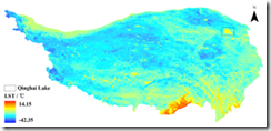
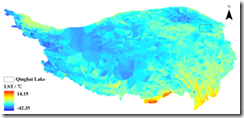
本软件实现了一种新的基于相似性原理的MODIS陆表温度(LST)的插值方法。这种LST数据空间插值方法利用具有相似温度变化特征的已知LST像元集合推算缺失的LST。在青藏高原的案例表明传统的地统计方法基本无法处理大范围连续的数据丢失(比如因为云),而本方法明显优于传统方法,可能较合理的得到缺失LST。此方法尤其适用于大范围山地区域。

This tool implements a new interpolation method for MODIS land surface temperature (LST) following the theory of similarity. It estimates the missing LST pixels by known LST pixel sets which bear similar characteristics of LST variation as the missing pixels. A case study on the Qinghai Tibet plateau has already been carried out, showing its obvious advantages over the traditional geostatistic methods, the latter was unable to do with a large area and temporally continuous data missing situations. This approach is especially good for a study area with a large area and mountainous terrain.

6704d1efb515c7a26d93914d72b14448

fig 1a, with this approach

315bdc690406652281a46f305a2e6697

fig 1b, with Kriging

Continue reading

Matlab科学数据处理:如何补上缺失的时间序列

Matlab科学数据处理:如何补上缺失的时间序列

Zhuotong Nan (南卓铜, [email protected])

问题提出

假设我们有一个时间序列文件,内容如下

286880 19480223 -5.7

286880 19480227 10.8

286880 19480229 7.7

286880 19480301 -15.7

286880 19480302 3.2

286880 19480303 7.7

286880 19480305 21.2

第一列是站点名,第二列是时间信息,第三列是温度值。时间并不连接,我们经常需要把时间补全,这些时间上的观测以缺失值(比如999.9)替代。即,我们希望是,

286880 19480223 -5.7

286880 19480224 999.9

286880 19480225 999.9

286880 19480226 999.9

286880 19480227 10.8

286880 19480228 999.9

286880 19480229 7.7

286880 19480301 -15.7

286880 19480302 3.2

286880 19480303 7.7

286880 19480304 999.9

286880 19480305 21.2

那么在matlab里要如何实现呢。

基本思路 Continue reading

将Global AVHRR NDVI 3g转换为ESRI ASCII Grid栅格的Matlab代码

我在前面的帖子(previous post)介绍了用ArcGIS读取GIMMS AVHRR NDVI 3g格式的数据文件的方法,但并不十分好用。所以写了一点代码,用于方便的将之转换为ESRI ASCII Grid栅格,后者可以很容易的被GIS软件支持。

从这个帖子可以下载到相关的代码和样例ndvi3g数据。

注意运行代码需要 Matlab的支持。

Purpose: Convert GIMMS Global AVHRR NDVI 3g files to ESRI ASCII Grid, which is very easy to be accessed with popular GIS software.
Author: Zhuotong Nan ([email protected])
Web: https://nanzt.info
Date: Sep 11,2014

Last update: Nov 3,2014

Please distribute codes with this header attached.

Usage:

type convert_ndvi3g_ascii in Matlab to run

Open convert_ndvi3g_ascii.m, modify the ndvi3gfl variable to make it point to the ndvi 3g file you wanto to convert.

After run, three grid files will be created. One is the grid
corresponding to the 3g data file, the other is the ndvi grid extracted from the 3g data file, and the last one is its associated flag grid.

Files included with this code:

  • convert_ndvi3g_ascii.m, the main matlab script
  • geo82dec15a.n07-VI3g, example avhrr ndvi 3g file
  • geo82dec15a.n07-VI3g.asc, ascii grid file corresponding to geo82dec15a.n07-VI3g
  • geo82dec15a.n07-VI3g.ndvi.asc, ascii grid file of the extracted ndvi
  • geo82dec15a.n07-VI3g.flag.asc, grid file of associated flags
  • header.txt, esri grid header information, used in code
  • Readme.txt, this file.

The meaning of the FLAG:
FLAG = 7 (missing data)
FLAG = 6 (NDVI retrieved from average seasonal profile, possibly snow)
FLAG = 5 (NDVI retrieved from average seasonal profile)
FLAG = 4 (NDVI retrieved from spline interpolation, possibly snow)
FLAG = 3 (NDVI retrieved from spline interpolation)
FLAG = 2 (Good value)
FLAG = 1 (Good value)

Nov 3, 2014
Fix bugs that wrongly computing ndvi.asc and flag.asc

Sep 11, 2014
Initial version

Download codes (9,875KB); Link2 (Baidu)

78ae077b84d7455913382971da7731ef  soft.ndvi3g.11032014.zip

Download codes (6,483KB)

MD5:  006d2d630a5c94f3ca629fc9f751d7f1  soft.ndvi3g.zip

多元回归 / 多元拟合matlab实现

MatLab内置了很多拟合的功能,比如分布、指数、多项式等拟合。对应的函数是fit。基本用法是:

cfun = fit(xdata, ydata, libname)

其中xdata是自变量x序列,ydata是因变量,libname 是模型名,比如’power1’是 y= a* x ^b 形式,Matlab内置了很多模型,可以从帮助文档里看到。对于这些拟合,MatLab有个图形工作叫 cftool,在命令行里敲入可以打开。

然而我们有时候需要做二元、多元拟合。

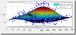
二元拟合,即使用模型 z = f(x, y),在MatLab也叫面拟合 (Surface fitting),有专门的图形工具 sftool,命令敲入sftool可以打开。

但如果是多元拟合,这时我们需要懂一点代码的工作。

其实不管一元、二元,代码级别是一致的。使用的都是fit命令。

对于使用 y = a* x^b这样内置的指数一元拟合,我们可以看到其libname 叫’power1’。所以采用以下命令:

cfun = fit(x, y, ‘power1’)

即从已知x、序列是得到拟合函数。coeffvalues(cfun)可以得到拟合参数,即这个例子里的a、b。如果还需要得到拟合指标,使用[cfun gof] = fit(x,y, ‘power1’),返回的gof包括了R squre、RMSE等多种指标。

对于二元拟合,比如 使用 z= a + b*sin(m*pi*x*y) + c*exp(-(w*y)^2模型进行拟合,采用类似的代码:

ft = fittype( ‘a + b*sin(m*pi*x*y) + c*exp(-(w*y)^2)’, ‘indep’, {‘x’, ‘y’}, ‘depend’, ‘z’ );

opts = fitoptions( ft );

opts.Display = ‘Off’;

opts.Lower = [-Inf -Inf -Inf -Inf -Inf];

opts.StartPoint = [0.741864193163802 0.681571628918889 0.811658042300087 0.275716137656952 0.738979809065491];

opts.Upper = [Inf Inf Inf Inf Inf];

opts.Weights = zeros(1,0);

[fitresult, gof] = fit( [x, y], z, ft, opts );

其中fittype自定义了需要的二元函数。其中’indep’指明自变量、’depend’指明因变量。即通过fittype构造一个二元拟合模型,说明其中的自变量和因变量,定义拟合的选项,这些选项经常可以不要专门指定,采用默认的即可。然后使用 fit的扩展形式得到拟合函数。

对于多元拟合,一个函数是 regress多元线性回归,另一个是nlinfit 非线性回归。两者都在statistic toolbox里。regress的基本形式是

b = regress(y, X)

其中X是多个自变量,y是因变量。

对于多元非线性拟合,可以使用nlinfit,基本形式是:

beta = nlinfit(X,Y,modelfun,beta0)

其中modelfun构造非线性多元模型,比如以下例子:

beta = nlinfit(X,y,@hougen,beta0)

使用一个hougen函数作为拟合模型,这个函数可以自行构建。

Matlab也提供了非线性多元拟合的图形化工具nlintool。

此外类似的还有 fitnlm函数提供了类似nlinfit的非线性回归,用法与nlinfit类似,但对返回结果进行包装,可以更简便的使用诸如predict等函数对非线性模型进行预报计算。

Image(1)

MATLAB之正则表达式

([email protected])

这种文本文件很大,比如我测试的样本文件,一共1281889行,约61.7MB,其余文件有超过120M的。对于这种大文件,手工处理十分费劲,必须要写代码处理。

因此流程很简单:

  1. 找到第一个Cyclic Acquisition,将此前的全部行,放到比如字符串s1;
  2. 从s1中移去preload data部分(包括头信息和数据),得到s2;
  3. 从s2中移去hold data 剖分(包括头信息和数据),得到s3;
  4. 从s3中移去多余的Data Acquisition头信息,即只保留第一个Data Acquisition头信息,得到s4;
  5. 将s4输出到a_static.dat。
  6. 得到1-14行头信息;
  7. 得到第一个Cyclic Acquisition及以后的全部行
  8. 合并6、7得到的字符串
  9. 输出到a_dynamic.dat。

所以这里的关键是如何得到我们需要的字符串,或者将某些字符串移去。一个很好的办法是使用正则表达式(regular expression),MATLAB里的函数是regexp。另外有regexprep是用于将匹配上的字符串用指定字符串替代,比如应用在步骤2、3、4。

本例演示了在MATLAB里使用正则表达式从文本中提取或替换子串。演示了regexp、regexprep的使用。本例也演示了对多个文件批处理的实现。

完整见附件PDF。

在超算上执行Matlab程序

新发展了一个算法,对MODIS LST进行重建。对象是青藏高原250sq km,共2.7M多个点。工作量十分大。写了Matlab代码。在实验室工作站进行 parallel运行,开了8个labs,每一幅大约花费 3-5小时。希望计算2005年一年的day和night LST。计算时间不能接受。

研究所部署有曙光5000大型机。LSF管理系统。在个人用户下(不一定需要系统权限,一般用户即可)安装了Matlab 2010a,MatlabRoot是 /public1/CAS/wanglx/matlab1。Putty连接到超算后,执行./matlab1/bin/matlab,提示glibc 不支持,当前版本是 glibc 2.4,2010a支持的版本是 2.7,需要用户输入y 才能继续进入到matlab。需要对oscheck.sh进行crack,否则以后的bsub提交系统会有问题。vi $Matlabroot/bin/util/oscheck.sh进去后,注释掉584行 read ans(前面添加 #)。其后插入一行 ans = ‘y’。:w! 保存(加!是因为文件是只读),:q退出 vi。

安装XME,远程连接到超算,启动matlab,在Parallel菜单里配置 default configuration。配置一个合适的叫lsfconfig。设为default。注意在字符界面下是无法配置 defaultParallelConfig的。

使用parallel configuration是为了使用matlabpool 进行自动的分割和管理。否则自己得使用设定scheduler, job, 和task 还得自己管理输入和输出。比较麻烦一些。matlabpool 可以跟 parfor等连接起来使用,对于我们面临的任务简单的for循环十分适用。

退出xme。以 matlab -nodisplay进去,调用 interp_lst2 执行,以high 队列进去,自动连接到 256个labs进行计算。在configuration时配置 submitarguments 为 -qhigh。

interp_lst2的结构如下:

function interp_lst2

%set up some variables and reading data in from files

matlabpool open lsfconfig 64

for i=1:length(lst_data_fns)

decompose2_func(interp_image_fn, lst_dir, ref_dir, output_dir, …
dem, slope, aspect);

end

matlabpool close

function decompose2_func(…)

%set up variables

parfor i=1:interp_count

end

%posterior procedures

使用matlab拟合Gamma分布

南卓铜 ([email protected])

任务描述: 有一批数据,需要将其histogram拟合成Gamma分布,histogram分20个bin,从0到100。结果如下图所示:

hist_dist_final

实现步骤:

1. 装载数据进来,数据文件是data.for.hist.txt,文件结构是一列无header的数据,共43个数据。

>> data=load(‘data.for.hist.txt’)

data是43×1的矢量。

2. 打开distribution fitting tool

>> dfittool

选择Display type为Density(PDF)。点击Data…,弹出Data对话框。

在此对话框内,设置Data为 ‘data’矢量,Censoring和Frequency为 none。设置data set name为dataset,然后点击 Create Data Set。

点击Set Bin Rules,设置Bin width为5。其余不变,OK确认关闭Set Bin Rules。这时,我们将data的histogram设置为每个bin长度为5。在不同的应用里,bin根据具体情况调整。关闭Data对话框。

3. Gamma拟合

点击New Fit…,在New Fit对话框里选择Data为dataset,Distribution为Gamma,点击Apply进行拟合。点击Close关闭New Fit对话框。

此时,看到下图的效果:

image

我们需要修改它的X域,使之匹配我们的histogram的X最大值100。点击Tools菜单下的Axes Limit Control,将X Lower Limit和X Upper Limit更改为 0和100。

image

4. 导出成figure

使用File菜单下的Print to Figure导出成figure。对figure进行必要修改。

>>figure(1)  (注,如果已经打开多个figure窗口,导出的figure序号可能不是1而是其它数字,注意figure窗口标题上的Figure n里的n)
>>legend hide
>>xlabel ‘1/32 degree, mm/day’
>>ylabel ‘Frequency’

此时效果如下,

image

5. 修改figure格式

设置figure为Tools-> edit plot状态,打开View->Property Editor。

将histogram的plot type从line改成Area,配置合适的face color和edge color。

将x轴的范围X Limits设置为0 to 100。

image

这时,histogram压着拟合曲线,选择拟合曲线,右键Cut后,再Paste进来,可以将拟合曲线带到最上面。

6. 修改数据

注意到目前为止,Y轴仍是Density。我们需要将Y坐标修改为Frequency(或者count)。Count=Density x bin width x data count,这里bin width是5,data count是43。因此,我们需要对Ydata乘以5×43=215。

选择拟合曲线,

>>ydata=get(gco,’YData’)
>>ydata_215 = ydata*215
>>set(gco,’YDATA’,ydata_215)

选择histogram,

>>set(gco,’YDATA’,get(gco,’YDATA’)*215)

修改xlim和ylim

>>ylim([0 10])
>>xlim([0 100])

将figure还原为非编辑状态。Tools->Edit Plot,并关闭Property editor。

image

以上步骤中数次修改xlim和ylim,并不是每次都需要,这里仅是为了演示需要。

7. 保存图形

>>print -dpng ‘histogram_dist.png’

在figure对话框的File-> Save As…保存为MATLAB Figure(.fig),以后可以通过File->Open…打开。

结论

本文演示了如何使用Matlab对数据的histogram使用Gamma分布进行拟合。介绍了matlab的常用命令,Distribution Fitting Tool,figure的格式化编辑功能,对figure对像数据的修改等。也介绍了比如如何调整figure里对像的z-order等实用技巧。

data.for.hist.txt